Posted 23 April 2019
A little over three years ago I developed an effective technique for detecting when Wall-E2, my autonomous wall-following robot, had gotten itself stuck and needed to back up and try again. The technique, described in that post, was to continuously calculate the mathematical variance of the last N forward distance measurements from the onboard LIDAR module. When Wall-E2 is moving, the forward distances increase or decrease, and the calculated variance is quite high (generally in the thousands). However, when it gets stuck the distances remain steady, and then the variance decreases rapidly to near zero. Setting a reasonable threshold allows Wall-E2 to figure out it is stuck on something and take appropriate action to recover.
The above arrangement has worked very well for the last three years, but recent developments and some nagging concerns prompted me to re-examine this feature.
Computational Load:
When I first added the variance calculation routine, there was very little else going on in Wall-E2’s brain; ping left, ping right, LIDAR forward, calc variance, adjust motor speeds, repeat. Since then, however, I have added a number of different sensor packages, all of which add to the computational load in one way or another. I began to be concerned that I might be about to exceed the current 100 mSec time budget.
Performance Problems:
Although the LIDAR/Variance technique has performed very well, there were still occasions where Wall-E2’s behavior indicated something was wrong; either he would think he was stuck when he obviously wasn’t, or it would take too long to detect a stuck condition, or other random glitches. This didn’t happen very often, but just enough to put me on notice that something wasn’t quite right.
Brute Force vs Incremental Variance Calculation:
I could only think of two ways to address the computational load; reduce the size of the array of LIDAR distances used, or reduce the time required for each computation. The original size selection of 50 measurements was sort of based on the idea that it would take about 5 seconds for a 50-entry array to be completely refreshed at the current 10Hz loop frequency. This means that Wall-E2 should be able to detect a stuck condition about 5 seconds after it happens. Decreasing the array size would decrease the detection time more or less linearly, but would probably also increase the chances of a false positive. The other alternative would be to find a way to speed up the variance calculation itself.
Variance is a measure of the variability of a dataset, and is defined as:
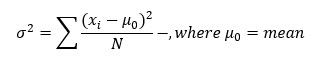
The current algorithm for computing the variance is a ‘Brute Force’ method that loops through the entire array of LIDAR distance values twice – once for computing the mean, and then again to compute the squared-difference term, before subtracting the squared mean from the squared difference term to get the final variance value, as shown below:
|
1 2 3 4 5 6 7 8 9 10 11 12 13 14 15 16 |
//calc new 'brute force' mean long sum = 0; for (int i = 0; i < DIST_ARRAY_SIZE; i++) { sum += aDistArray[i]; //adds in rest of values } float brute_mean = (float)sum / (float)DIST_ARRAY_SIZE; // Step2: calc new 'brute force' variance float sumsquares = 0; for (int i = 0; i < DIST_ARRAY_SIZE; i++) { sumsquares += (aDistArray[i] - brute_mean)*(aDistArray[i] - brute_mean); } double brute_var = sumsquares / DIST_ARRAY_SIZE; |
This works fine, but is computationally clunky. With a 50-element array, this computation takes around 1.5 mSec. This is only about 1.5% of the 100 mSec time window for a 10Hz cycle time, but still…
Starting from a slightly different definition of the variance calculation
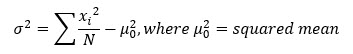
and then expanding, manipulating algebraically and then recombining, we arrive at an incremental version of the variance formula, as shown below:
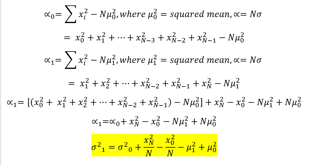
Incremental version of the variance expression
And this is implemented in the code section shown below:
|
1 2 3 4 5 6 7 8 9 10 |
double inc_mean = last_incmean - (float)oldestDistVal / DIST_ARRAY_SIZE + (float)newdistval / DIST_ARRAY_SIZE; unsigned long olddist_squared = oldestDistVal * oldestDistVal; unsigned long newdist_squared = newdistval * newdistval; double last_incmean_squared = last_incmean * last_incmean; double inc_mean_squared = inc_mean * inc_mean; double inc_var = last_incvar + ((float)newdist_squared / DIST_ARRAY_SIZE) - ((float)olddist_squared / DIST_ARRAY_SIZE) + last_incmean_squared - inc_mean_squared; |
The incremental calculation doesn’t use any loops and therefore is quite a bit faster, for no loss in accuracy. For a 50-element array as above, the incremental calculation takes only about 220 uSec, or about 7-8 times faster than the ‘brute force’ technique.
As a side-benefit of changing from the ‘brute force’ to the incremental technique, I also discovered the reason Wall-E2 was displaying occasional odd behavior. The sonar ping measurements have a maximum value of 200 cm, which fits nicely into a 8-bit ‘byte’ data type. However, the LIDAR front distance sensor goes out to 400 cm, which doesn’t. Unfortunately, I had defined the forward distance array as an array of ‘byte’ values, which meant that everything worked fine as long as the reported distance was less than 255 cm, but not so much for distances over that value. Fixing this problem turned out not to be as simple as changing the array definition from ‘byte’ to uint16_t, as then I ran into numerical overflow problems in the incremental variance calculation because of the squaring operations involved. Due to the way the compiler operates, it isn’t sufficient to cast the result of uint16_t * uint16_t, to uint32_t, as the overflow happens before the cast. To avoid this problem, the individual terms need to be uint32_t before the multiplication occurs. Once this was done, all the results settled down to what they should be, and now correct results are obtained for the full range of possible distance values. Shown below is an Excel plot of a test run performed using simulated input values from 100 to 400 (anything above 255 used to cause overrun problems)
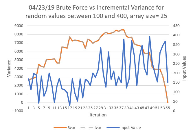
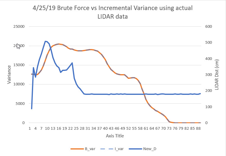
As can be seen in the above plot, the ‘brute force’ and incremental methods both produce identical outputs, but the incremental method is 7-8 times faster.
Shown below is the same setup, but this time the input data is actual LIDAR data from the robot
03 May 2022 Update:
As part of my ongoing work to integrate charging station homing into my new Wall-E3 autonomous wall-following robot, I discovered that the ‘stuck detection’ routine wasn’t working anymore. Upon investigation I found that the result returned by the above incremental variance calculation wasn’t decreasing to near zero as expected when the robot was stuck; in fact, the calculated variance stayed pretty constant at about 10,000 – how could that be? After beating on this for a while, I realized that if the four terms to the right of the previous incremental variance calculation add to near zero, which they will if the array contents are constant, then the new calculated variance will be the same as the old calculated variance. So, if the ‘previous variance’ number starts out wrong, it will stay wrong, and the ‘stuck’ flag will never be raised – oops!
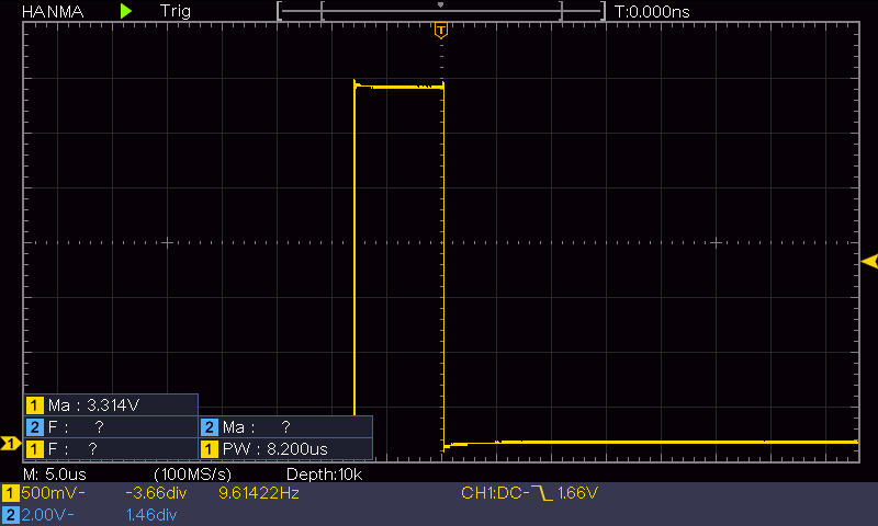
I started thinking again about why I changed from the ‘brute force’ method to the incremental method in the first place. The reason at the time was my concern that the brute force method might eat up too much of the available loop cycle time, but now that I have changed the processor from an Arduino MEGA2560 to a Teensy 3.5, that might not be applicable anymore. So I replaced the incremental algorithm with the brute force one, and instrumented the block with a hardware pin to actually measure the time required to compute the variance. As shown below, this is approximately 8μSec, insignificant compared to the 100 mSec tracking loop duration.
Stay tuned,
Frank