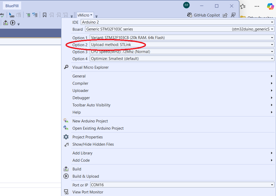
Board Properties
name=Generic STM32F103C series
vid.0=0x1EAF
pid.0=0x0004
build.variant=generic_stm32f103c
build.vect=VECT_TAB_ADDR=0x8002000
build.core=maple
build.board=GENERIC_STM32F103C
build.error_led_port=GPIOC
build.error_led_pin=13
upload.use_1200bps_touch=false
upload.file_type=bin
upload.auto_reset=true
upload.tool=maple_upload
upload.protocol=maple_dfu
menu.device_variant.STM32F103C8=STM32F103C8 (20k RAM. 64k Flash)
menu.device_variant.STM32F103C8.build.cpu_flags=-DMCU_STM32F103C8
menu.device_variant.STM32F103C8.build.ldscript=ld/jtag_c8.ld
menu.device_variant.STM32F103C8.upload.maximum_size=65536
menu.device_variant.STM32F103C8.upload.maximum_data_size=20480
menu.device_variant.STM32F103CB=STM32F103CB (20k RAM. 128k Flash)
menu.device_variant.STM32F103CB.build.cpu_flags=-DMCU_STM32F103CB
menu.device_variant.STM32F103CB.build.ldscript=ld/jtag.ld
menu.device_variant.STM32F103CB.upload.maximum_size=131072
menu.device_variant.STM32F103CB.upload.maximum_data_size=20480
menu.upload_method.DFUUploadMethod=STM32duino bootloader
menu.upload_method.DFUUploadMethod.upload.protocol=maple_dfu
menu.upload_method.DFUUploadMethod.upload.tool=maple_upload
menu.upload_method.DFUUploadMethod.build.upload_flags=-DSERIAL_USB -DGENERIC_BOOTLOADER
menu.upload_method.DFUUploadMethod.build.vect=VECT_TAB_ADDR=0x8002000
menu.upload_method.DFUUploadMethod.build.ldscript=ld/bootloader_20.ld
menu.upload_method.DFUUploadMethod.upload.usbID=1EAF:0003
menu.upload_method.DFUUploadMethod.upload.altID=2
menu.upload_method.serialMethod=Serial
menu.upload_method.serialMethod.upload.protocol=maple_serial
menu.upload_method.serialMethod.upload.tool=serial_upload
menu.upload_method.serialMethod.build.upload_flags=-DCONFIG_MAPLE_MINI_NO_DISABLE_DEBUG
menu.upload_method.STLinkMethod=STLink
menu.upload_method.STLinkMethod.upload.protocol=STLink
menu.upload_method.STLinkMethod.upload.tool=stlink_upload
menu.upload_method.STLinkMethod.build.upload_flags=-DCONFIG_MAPLE_MINI_NO_DISABLE_DEBUG=1 -DSERIAL_USB -DGENERIC_BOOTLOADER
menu.upload_method.BMPMethod=BMP (Black Magic Probe)
menu.upload_method.BMPMethod.upload.protocol=gdb_bmp
menu.upload_method.BMPMethod.upload.tool=bmp_upload
menu.upload_method.BMPMethod.build.upload_flags=-DCONFIG_MAPLE_MINI_NO_DISABLE_DEBUG
menu.upload_method.jlinkMethod=JLink
menu.upload_method.jlinkMethod.upload.protocol=jlink
menu.upload_method.jlinkMethod.upload.tool=jlink_upload
menu.upload_method.jlinkMethod.build.upload_flags=-DCONFIG_MAPLE_MINI_NO_DISABLE_DEBUG=1 -DSERIAL_USB -DGENERIC_BOOTLOADER
menu.upload_method.HIDUploadMethod=HID bootloader 2.0
menu.upload_method.HIDUploadMethod.upload.tool=hid_upload
menu.upload_method.HIDUploadMethod.build.upload_flags=-DSERIAL_USB -DGENERIC_BOOTLOADER
menu.upload_method.HIDUploadMethod.build.vect=VECT_TAB_ADDR=0x8001000
menu.upload_method.HIDUploadMethod.build.ldscript=ld/hid_bootloader.ld
menu.cpu_speed.speed_72mhz=72Mhz (Normal)
menu.cpu_speed.speed_72mhz.build.f_cpu=72000000L
menu.cpu_speed.speed_48mhz=48Mhz (Slow - with USB)
menu.cpu_speed.speed_48mhz.build.f_cpu=48000000L
menu.cpu_speed.speed_128mhz=Overclocked 128Mhz NO USB SERIAL. MANUAL RESET NEEDED TO UPLOAD
menu.cpu_speed.speed_128mhz.build.f_cpu=128000000L
menu.opt.osstd=Smallest (default)
menu.opt.o1std=Fast (-O1)
menu.opt.o1std.build.flags.optimize=-O1
menu.opt.o1std.build.flags.ldspecs=
menu.opt.o2std=Faster (-O2)
menu.opt.o2std.build.flags.optimize=-O2
menu.opt.o2std.build.flags.ldspecs=
menu.opt.o3std=Fastest (-O3)
menu.opt.o3std.build.flags.optimize=-O3
menu.opt.o3std.build.flags.ldspecs=
menu.opt.ogstd=Debug (-g)
menu.opt.ogstd.build.flags.optimize=-Og
menu.opt.ogstd.build.flags.ldspecs=
vm.debug.class_type=VM_DBT_USBSERIAL
vm.debug.main_port_name=Serial
tools.openocd.debug.build.openocdscript=target/stm32f1x.cfg
menu.upload_method.f2232h=F2232H Dual RS232 + OpenOCD (vMicro)
menu.upload_method.f2232h.upload.tool=ftdiocd
menu.upload_method.f2232h.upload.openocddebugger=ftdi/minimodule-lowcost.cfg
menu.upload_method.cjmcuf2232h=F2232H Single RS232 + OpenOCD (vMicro)
menu.upload_method.cjmcuf2232h.upload.tool=ftdiocd
menu.upload_method.cjmcuf2232h.upload.openocddebugger=ftdi/um232h.cfg
menu.upload_method.ft2232mm=JLink + OpenOCD (vMicro)
menu.upload_method.ft2232mm.upload.tool=jlinkocd
menu.upload_method.ft2232mm.upload.openocddebugger=jlink.cfg
menu.upload_method.stlinkv2=STLink v2 + OpenOCD (vMicro)
menu.upload_method.stlinkv2.upload.tool=openocd
menu.upload_method.stlinkv2.upload.openocddebugger=stlink.cfg
menu.upload_method.stlinkv21=STLink v2.1 + OpenOCD (vMicro)
menu.upload_method.stlinkv21.upload.tool=openocd
menu.upload_method.stlinkv21.upload.openocddebugger=stlink.cfg
menu.upload_method.bmp=Black Magic + GDB (vMicro)
menu.upload_method.bmp.upload.tool=vmbmp
menu.upload_method.bmp.upload.openocddebugger=
menu.upload_method.daplink=DAPLink + OpenOCD (vMicro)
menu.upload_method.daplink.upload.tool=daplink
runtime.ide.path=c:\program files\microsoft visual studio\2022\community\common7\ide\extensions\jbmj4m1q.esc\Micro Platforms\visualmicro\ide
runtime.os=windows
build.system.path=c:\Users\Frank\AppData\Local\Arduino15\packages\stm32duino\hardware\STM32F1\2022.9.26\system
runtime.ide.version=108010
target_package=stm32duino
target_platform=STM32F1
runtime.hardware.path=c:\Users\Frank\AppData\Local\Arduino15\packages\stm32duino\hardware\STM32F1
originalid=genericSTM32F103C
_id=genericSTM32F103C
intellisense.tools.path={runtime.tools.arm-none-eabi-gcc.path}
intellisense.include.paths={runtime.tools.CMSIS.path}/CMSIS/Core/Include/;{intellisense.tools.path}\arm-none-eabi;{intellisense.tools.path}\arm-none-eabi\include;{intellisense.tools.path}\arm-none-eabi\include\c++\9.2.1\arm-none-eabi;{intellisense.tools.path}\arm-none-eabi\include\c++\9.2.1;{intellisense.tools.path}\arm-none-eabi\include\c++\9.2.1\tr1;{intellisense.tools.path}\arm-none-eabi\include\sys;{intellisense.tools.path}\arm-none-eabi\include\c++\9.2.1\arm-none-eabi\bits; {intellisense.tools.path}\lib\gcc\arm-none-eabi\9.2.1\include;{intellisense.tools.path}\arm-none-eabi\include\c++\4.8.3\arm-none-eabi;{intellisense.tools.path}\arm-none-eabi\include\c++\4.8.3;{intellisense.tools.path}\arm-none-eabi\include\c++\4.8.3\tr1;{intellisense.tools.path}\arm-none-eabi\include\c++\4.8.3\arm-none-eabi\bits;{intellisense.tools.path}\lib\gcc\arm-none-eabi\4.8.3\include;{vm.intellisense.add-paths}
upload.8dot3=false
tools.gdb.pre_init.tool=openocd
tools.gdb.cmd=arm-none-eabi-gdb.exe
tools.gdb.path={runtime.tools.arm-none-eabi-gcc.path}/bin
tools.gdb.pattern="{path}/{cmd}" -interpreter=mi -d "{build.project_path}"
tools.gdb.openocd.cmd=bin/openocd.exe
tools.gdb.openocd.path={runtime.vm.ide.tools.openocd.path}
tools.gdb.openocd.params.verbose=-d2
tools.gdb.openocd.params.quiet=-d0
tools.gdb.openocd.pattern="{path}/{cmd}" -l "{{build.path}/{build.project_name}_DebugOpenOCD.log}" -s "{path}/scripts/" -f "{path}/scripts/{build.openocdscript}"
tools.openocd.debug.path={runtime.tools.openocd-0.10.0.20200213.path}
tools.openocd.debug.cmd=bin/openocd.exe
tools.openocd.debug.cmd.windows=bin/openocd.exe
tools.openocd.debug.params.verbose=-d2
tools.openocd.debug.params.quiet=-d0
tools.openocd.initCmd=-c "init; reset halt"
vs-cmd.Debug.AttachtoProcess.tools.openocd.initCmd=-c "init"
tools.openocd.debug.args={params.verbose} -l "{{build.path}/{build.project_name}_DebugOpenOCD.log}" -s"{path}/scripts/" -f "{path}/scripts/interface/{build.openocddebugger}" -f "{path}/scripts/{build.openocdscript}" {initCmd}
tools.openocd.debug.address=localhost:3333
tools.bmp_upload.debug.args=-nh -b 115200 -ex "target extended-remote \.\{serial.debug.port}" -ex "monitor swdp_scan" -ex "attach 1"
tools.f2232h.vmserver.targetCmd=-c "transport select swd" -c "ftdi_layout_signal SWD_EN -data 0" -f "{tools.openocd.debug.build.openocdscript}"
tools.cjmcuf2232h.vmserver.targetCmd=-c "transport select swd" -c "ftdi_layout_signal SWD_EN -data 0" -f "{tools.openocd.debug.build.openocdscript}"
tools.f2232mm.vmserver.targetCmd=-c "transport select swd" -c "ftdi_layout_signal SWD_EN -data 0" -f "{tools.openocd.debug.build.openocdscript}"
tools.jlink.vmserver.targetCmd=-c "transport select swd" -f "{tools.openocd.debug.build.openocdscript}"
tools.stlinkv2.vmserver.targetCmd=-f "{tools.openocd.debug.build.openocdscript}"
tools.stlinkv2.debug.args=-ex "flushregs" -ex "continue"
tools.daplink.vmserver.targetCmd=-c "transport select swd" -f "{tools.openocd.debug.build.openocdscript}"
debug_menu.hwdebugger.bmp=Black Magic (External)
debug_menu.hwdebugger.bmp.debug.tool=bmp_upload
meta_bmp.sentence=This debugger requires the 20-pin ribbon cable to link to your target, see connections below
meta_bmp.comment=Ensure the COM Port for the Black Magic is selected before attaching the Debugger. Set vMicro > Debugger > 'Compiler Optimization' to 'No Project', 'No Project + Libraries' or 'None' when debugging. (NOTE: Changing the optimization setting for this platform might cause compilation errors with certain code such as HardwareSerial.)
meta_bmp.image.connect=https://www.visualmicro.com/pics/Debug-Help-STM32-BMP-Connections.png
meta_bmp.image.operation=https://www.visualmicro.com/pics/Debug-Break-STM32-BMP-VSOnly.png
meta_bmp.reference.usage.url=https://www.visualmicro.com/page/STM32-Debugging.aspx
debug_menu.hwdebugger.f2232h=F2232H Dual RS232
debug_menu.hwdebugger.f2232h.debug.tool=f2232h
meta_f2232h.sentence=This debugger will require some wiring to connect it to your target STM32 board
meta_f2232h.comment=Wiring can be found in the below image, and the 'https://zadig.akeo.ie/' tool is required to replace the USB Driver on Interface 0 with 'WinUSB'. Set vMicro > Debugger > 'Compiler Optimization' to 'No Project', 'No Project + Libraries' or 'None' when debugging. (NOTE: Changing the optimization setting for this platform might cause compilation errors with certain code such as HardwareSerial.)
meta_f2232h.image.connect=https://www.visualmicro.com/pics/Debug-Break-STM32-FT2232H-Connections.png
meta_f2232h.reference.usage.url=https://www.visualmicro.com/page/STM32-Debugging.aspx
debug_menu.hwdebugger.cjmcuf2232h=F2232H Single RS232
debug_menu.hwdebugger.cjmcuf2232h.debug.tool=cjmcuf2232h
meta_cjmcuf2232h.sentence=This debugger will require some wiring to connect it to your target STM32 board
meta_cjmcuf2232h.comment=Wiring can be found in the below image, and the 'https://zadig.akeo.ie/' tool is required to replace the USB Driver on Interface 0 with 'WinUSB'. Set vMicro > Debugger > 'Compiler Optimization' to 'No Project', 'No Project + Libraries' or 'None' when debugging. (NOTE: Changing the optimization setting for this platform might cause compilation errors with certain code such as HardwareSerial.)
meta_cjmcuf2232h.image.connect=https://www.visualmicro.com/pics/Debug-Break-STM32-CJMCU2232H-Connections.png
meta_cjmcuf2232h.reference.usage.url=https://www.visualmicro.com/page/STM32-Debugging.aspx
debug_menu.hwdebugger.f2232mm=F2232 MiniModule
debug_menu.hwdebugger.f2232mm.debug.tool=f2232mm
meta_f2232mm.sentence=This debugger will require some wiring to allow it to function, and connect to your target STM32 board
meta_f2232mm.comment=Wiring can be found in the below image, and the 'https://zadig.akeo.ie/' tool is required to replace the USB Driver on Interface 0 with 'WinUSB'. Set vMicro > Debugger > 'Compiler Optimization' to 'No Project', 'No Project + Libraries' or 'None' when debugging. (NOTE: Changing the optimization setting for this platform might cause compilation errors with certain code such as HardwareSerial.)
meta_f2232mm.image.connect=https://www.visualmicro.com/pics/Debug-Help-STM32-FT2232MM-Connections.png
meta_f2232mm.image.operation=https://www.visualmicro.com/pics/Debug-Help-STM32-FT2232MM-VSOnly.png
meta_f2232mm.reference.usage.url=https://www.visualmicro.com/page/STM32-Debugging.aspx
debug_menu.hwdebugger.jlink=Segger J-Link
debug_menu.hwdebugger.jlink.debug.tool=jlink
meta_jlink.sentence=This debugger will require some wiring to connect it to your target STM32 board
meta_jlink.comment=Wiring can be found in the below image, and the 'https://zadig.akeo.ie/' tool is required to replace the USB Driver on Interface 0 with 'WinUSB'. Set vMicro > Debugger > 'Compiler Optimization' to 'No Project', 'No Project + Libraries' or 'None' when debugging. (NOTE: Changing the optimization setting for this platform might cause compilation errors with certain code such as HardwareSerial.)
meta_jlink.image.connect=https://www.visualmicro.com/pics/Debug-Help-STM32-Jlink-Connections.png
meta_jlink.image.operation=https://www.visualmicro.com/pics/Debug-Help-STM32-STM32-Jlink-VSOnly.png
meta_jlink.reference.usage.url=https://www.visualmicro.com/page/STM32-Debugging.aspx
debug_menu.hwdebugger.stlinkv21=STLink v2.1 (Onboard)
debug_menu.hwdebugger.stlinkv21.debug.tool=stlinkv2
meta_stlinkv21.sentence=This debugger is built onto the board, and requires both jumpers to be present on the STLINK/Board header
meta_stlinkv21.comment=Wiring can be found in the below image, and the 'https://zadig.akeo.ie/' tool is required to replace the USB Driver on Interface 0 with 'WinUSB'. Set vMicro > Debugger > 'Compiler Optimization' to 'No Project', 'No Project + Libraries' or 'None' when debugging. (NOTE: Changing the optimization setting for this platform might cause compilation errors with certain code such as HardwareSerial.)
meta_stlinkv21.image.connect=https://www.visualmicro.com/pics/Debug-Help-STM32-STlinkBuiltIn-Connections.png
meta_stlinkv21.image.operation=https://www.visualmicro.com/pics/Debug-Break-STM32-STlinkBuiltIn-VSOnly.png
meta_stlinkv21.reference.usage.url=https://www.visualmicro.com/page/STM32-Debugging.aspx
debug_menu.hwdebugger.stlinkv2=STLink v2 (External)
debug_menu.hwdebugger.stlinkv2.debug.tool=stlinkv2
meta_stlinkv2.sentence=This debugger requires the 20-pin ribbon cable to link to your target.
meta_stlinkv2.comment=Further info can be found in the below image, and the 'https://zadig.akeo.ie/' tool is required to replace the USB Driver on Interface 0 with 'WinUSB'. Set vMicro > Debugger > 'Compiler Optimization' to 'No Project', 'No Project + Libraries' or 'None' when debugging. (NOTE: Changing the optimization setting for this platform might cause compilation errors with certain code such as HardwareSerial.)
meta_stlinkv2.image.connect=https://www.visualmicro.com/pics/Debug-Help-STM32-STlink-Connections.png
meta_stlinkv2.image.operation=https://www.visualmicro.com/pics/Debug-Break-STM32-STlink-VSOnly.png
meta_stlinkv2.reference.usage.url=https://www.visualmicro.com/page/STM32-Debugging.aspx
debug_menu.hwdebugger.daplink=DAPLink
debug_menu.hwdebugger.daplink.debug.tool=daplink
meta_daplink.sentence=This debugger additional wiring to link to your target, see links below
meta_daplink.comment=Optionally set vMicro > Debugger > 'Compiler Optimization' to 'No Project', 'No Project + Libraries' or 'None' when debugging. (NOTE: Changing the optimization setting for this platform might cause compilation errors with certain code such as HardwareSerial.)
meta_daplink.image.connect=https://www.visualmicro.com/pics/Debug-Help-STM32-DAPLink-Connections.png
meta_daplink.image.operation=https://www.visualmicro.com/pics/Debug-Break-STM32-DAPLink-VSOnly.png
meta_daplink.reference.usage.url=https://www.visualmicro.com/page/STM32-Debugging.aspx
tools.openocd.upload.elf.message=****[vMicro]**** Uploading ELF :
tools.openocd.upload.path={runtime.tools.openocd-0.10.0.20200213.path}
tools.openocd.upload.cmd=bin/openocd.exe
tools.openocd.upload.cmd.windows=bin/openocd.exe
tools.openocd.upload.params.verbose=-d2
tools.openocd.upload.params.quiet=-d0
tools.openocd.upload.pattern="{upload.path}/{upload.cmd}" {upload.verbose} -s "{upload.path}/scripts/" -f "interface/{upload.openocddebugger}" -f "{upload.openocdscript}" -c "echo -n {{upload.elf.message}}" -c "reset_config; telnet_port disabled; program {{build.path}/{build.project_name}.elf} reset;reset_config;shutdown"
tools.openocd.upload.extra_params=
tools.openocd.upload.protocol=
tools.openocd.protocol=
tools.openocd.upload.openocdscript=target/stm32f1x.cfg
tools.jlinkocd.upload.elf.message=****[vMicro]**** Uploading ELF :
tools.jlinkocd.upload.path={runtime.tools.openocd-0.10.0.20200213.path}
tools.jlinkocd.upload.cmd=bin/openocd.exe
tools.jlinkocd.upload.cmd.windows=bin/openocd.exe
tools.jlinkocd.upload.params.verbose=-d2
tools.jlinkocd.upload.params.quiet=-d0
tools.jlinkocd.upload.pattern="{upload.path}/{upload.cmd}" {upload.verbose} -s "{upload.path}/scripts/" -f "interface/{upload.openocddebugger}" -c "transport select swd" -f "{upload.openocdscript}" -c "echo -n {{upload.elf.message}}" -c "reset_config; telnet_port disabled; program {{build.path}/{build.project_name}.elf} reset;reset_config;shutdown"
tools.jlinkocd.upload.extra_params=
tools.jlinkocd.upload.protocol=
tools.jlinkocd.protocol=
tools.jlinkocd.upload.openocdscript=target/stm32f1x.cfg
tools.ftdiocd.upload.elf.message=****[vMicro]**** Uploading ELF :
tools.ftdiocd.upload.path={runtime.tools.openocd-0.10.0.20200213.path}
tools.ftdiocd.upload.cmd=bin/openocd.exe
tools.ftdiocd.upload.cmd.windows=bin/openocd.exe
tools.ftdiocd.upload.params.verbose=-d2
tools.ftdiocd.upload.params.quiet=-d0
tools.ftdiocd.upload.pattern="{upload.path}/{upload.cmd}" {upload.verbose} -s "{upload.path}/scripts/" -f "interface/{upload.openocddebugger}" -c "transport select swd" -c "ftdi_layout_signal SWD_EN -data 0" -f "{upload.openocdscript}" -c "echo -n {{upload.elf.message}}" -c "reset_config; telnet_port disabled; program {{build.path}/{build.project_name}.elf} reset;reset_config;shutdown"
tools.ftdiocd.upload.extra_params=
tools.ftdiocd.upload.protocol=
tools.ftdiocd.protocol=
tools.ftdiocd.upload.openocdscript=target/stm32f1x.cfg
tools.vmbmp.upload.cmd=bin/arm-none-eabi-gdb.exe
tools.vmbmp.upload.cmd.windows=bin/arm-none-eabi-gdb.exe
tools.vmbmp.upload.path={runtime.tools.arm-none-eabi-gcc.path}
tools.vmbmp.upload.pattern={upload.path}/{upload.cmd} -nx -b 230400 -batch -ex "set confirm off" -ex "target extended-remote \.\{serial.port}" -ex "monitor swdp_scan" -ex "attach 1" -ex "load" -ex "compare-sections" -ex "kill" "{build.path}/{build.project_name}.elf" -ex "kill"
tools.daplink.upload.programCmd=-c "reset_config; telnet_port disabled; program {{build.path}/{build.project_name}.elf} reset;reset_config;shutdown"
tools.daplink.upload.targetCmd=-c "transport select swd" -f "{tools.openocd.upload.openocdscript}"
version=0.1.2
compiler.warning_flags=-w -DDEBUG_LEVEL=DEBUG_NONE
compiler.warning_flags.none=-w -DDEBUG_LEVEL=DEBUG_NONE
compiler.warning_flags.default=-DDEBUG_LEVEL=DEBUG_NONE
compiler.warning_flags.more=-Wall -DDEBUG_LEVEL=DEBUG_FAULT
compiler.warning_flags.all=-Wall -Wextra -DDEBUG_LEVEL=DEBUG_ALL
compiler.path={runtime.tools.arm-none-eabi-gcc.path}/bin/
compiler.c.cmd=arm-none-eabi-gcc
compiler.c.flags=-c -g {build.flags.optimize} {compiler.warning_flags} -std=gnu11 -MMD -ffunction-sections -fdata-sections -nostdlib --param max-inline-insns-single=500 -DBOARD_{build.variant} -D{build.vect} -DERROR_LED_PORT={build.error_led_port} -DERROR_LED_PIN={build.error_led_pin}
compiler.c.elf.cmd=arm-none-eabi-g++
compiler.c.elf.flags={build.flags.optimize} -Wl,--gc-sections {build.flags.ldspecs}
compiler.S.cmd=arm-none-eabi-gcc
compiler.S.flags=-c -g -x assembler-with-cpp -MMD
compiler.cpp.cmd=arm-none-eabi-g++
compiler.cpp.flags=-c -g {build.flags.optimize} {compiler.warning_flags} -std=gnu++11 -MMD -ffunction-sections -fdata-sections -nostdlib --param max-inline-insns-single=500 -fno-rtti -fno-exceptions -fno-use-cxa-atexit -DBOARD_{build.variant} -D{build.vect} -DERROR_LED_PORT={build.error_led_port} -DERROR_LED_PIN={build.error_led_pin}
compiler.ar.cmd=arm-none-eabi-ar
compiler.ar.flags=rcs
compiler.objcopy.cmd=arm-none-eabi-objcopy
compiler.objcopy.eep.flags=-O ihex -j .eeprom --set-section-flags=.eeprom=alloc,load --no-change-warnings --change-section-lma .eeprom=0
compiler.elf2hex.flags=-O binary
compiler.elf2hex.cmd=arm-none-eabi-objcopy
compiler.ldflags={build.flags.ldspecs}
compiler.size.cmd=arm-none-eabi-size
compiler.define=-DARDUINO=
build.f_cpu=72000000L
build.mcu=cortex-m3
build.common_flags=-mthumb -march=armv7-m -D__STM32F1__
build.variant_system_lib=libmaple.a
build.cpu_flags=-DMCU_STM32F103C8
build.hs_flag=
build.upload_flags=-DSERIAL_USB -DGENERIC_BOOTLOADER
build.flags.optimize=-Os
build.flags.ldspecs=--specs=nano.specs
build.extra_flags={build.upload_flags} {build.cpu_flags} {build.hs_flag} {build.common_flags}
compiler.c.extra_flags=
compiler.c.elf.extra_flags="-L{build.variant.path}/ld"
compiler.cpp.extra_flags=
compiler.S.extra_flags=
compiler.ar.extra_flags=
compiler.elf2hex.extra_flags=
compiler.libs.c.flags="-I{build.system.path}/libmaple" "-I{build.system.path}/libmaple/include" "-I{build.system.path}/libmaple/stm32f1/include" "-I{build.system.path}/libmaple/usb/stm32f1" "-I{build.system.path}/libmaple/usb/usb_lib"
recipe.c.o.pattern="{compiler.path}{compiler.c.cmd}" {compiler.c.flags} -mcpu={build.mcu} -DF_CPU={build.f_cpu} -DARDUINO={runtime.ide.version} -DARDUINO_{build.board} -DARDUINO_ARCH_{build.arch} {compiler.c.extra_flags} {build.extra_flags} {compiler.libs.c.flags} {includes} "{source_file}" -o "{object_file}"
recipe.cpp.o.pattern="{compiler.path}{compiler.cpp.cmd}" {compiler.cpp.flags} -mcpu={build.mcu} -DF_CPU={build.f_cpu} -DARDUINO={runtime.ide.version} -DARDUINO_{build.board} -DARDUINO_ARCH_{build.arch} {compiler.cpp.extra_flags} {build.extra_flags} {build.cpu_flags} {build.hs_flag} {build.common_flags} {compiler.libs.c.flags} {includes} "{source_file}" -o "{object_file}"
recipe.S.o.pattern="{compiler.path}{compiler.c.cmd}" {compiler.S.flags} -mcpu={build.mcu} -DF_CPU={build.f_cpu} -DARDUINO={runtime.ide.version} -DARDUINO_{build.board} -DARDUINO_ARCH_{build.arch} {compiler.S.extra_flags} {build.extra_flags} {build.cpu_flags} {build.hs_flag} {build.common_flags} {compiler.libs.c.flags} {includes} "{source_file}" -o "{object_file}"
recipe.ar.pattern="{compiler.path}{compiler.ar.cmd}" {compiler.ar.flags} {compiler.ar.extra_flags} "{archive_file_path}" "{object_file}"
recipe.c.combine.pattern="{compiler.path}{compiler.c.elf.cmd}" {compiler.c.elf.flags} -mcpu={build.mcu} "-T{build.variant.path}/{build.ldscript}" "-Wl,-Map,{build.path}/{build.project_name}.map" {compiler.c.elf.extra_flags} -o "{build.path}/{build.project_name}.elf" "-L{build.path}" -lm -lgcc -mthumb -Wl,--cref -Wl,--check-sections -Wl,--gc-sections -Wl,--unresolved-symbols=report-all -Wl,--warn-common -Wl,--warn-section-align -Wl,--warn-unresolved-symbols -Wl,--start-group {object_files} "{archive_file_path}" -Wl,--end-group
recipe.objcopy.eep.pattern=
recipe.objcopy.hex.pattern="{compiler.path}{compiler.elf2hex.cmd}" {compiler.elf2hex.flags} {compiler.elf2hex.extra_flags} "{build.path}/{build.project_name}.elf" "{build.path}/{build.project_name}.bin"
recipe.size.pattern="{compiler.path}{compiler.size.cmd}" -A "{build.path}/{build.project_name}.elf"
recipe.size.regex=^(?:\.text|\.data|\.rodata|\.text.align|\.ARM.exidx)\s+([0-9]+).*
recipe.size.regex.data=^(?:\.data|\.bss|\.noinit)\s+([0-9]+).*
recipe.output.tmp_file={build.project_name}.bin
recipe.output.save_file={build.project_name}.{build.variant}.bin
tools.maple_upload.cmd=maple_upload.bat
tools.maple_upload.cmd.windows=maple_upload.bat
tools.maple_upload.path={runtime.tools.stm32tools.path}/win
tools.maple_upload.path.macosx={runtime.tools.stm32tools.path}/macosx
tools.maple_upload.path.linux={runtime.tools.stm32tools.path}/linux
tools.maple_upload.path.linux64={runtime.tools.stm32tools.path}/linux
tools.maple_upload.upload.params.verbose=-d
tools.maple_upload.upload.params.quiet=
tools.maple_upload.upload.pattern="{path}/{cmd}" {serial.port.file} {upload.altID} {upload.usbID} "{build.path}/{build.project_name}.bin" "{runtime.ide.path}"
tools.serial_upload.cmd=serial_upload.bat
tools.serial_upload.cmd.windows=serial_upload.bat
tools.serial_upload.cmd.macosx=serial_upload
tools.serial_upload.path={runtime.tools.stm32tools.path}/win
tools.serial_upload.path.macosx={runtime.tools.stm32tools.path}/macosx
tools.serial_upload.path.linux={runtime.tools.stm32tools.path}/linux
tools.serial_upload.path.linux64={runtime.tools.stm32tools.path}/linux
tools.serial_upload.upload.params.verbose=-d
tools.serial_upload.upload.params.quiet=n
tools.serial_upload.upload.pattern="{path}/{cmd}" {serial.port.file} {upload.altID} {upload.usbID} "{build.path}/{build.project_name}.bin"
tools.stlink_upload.cmd=stlink_upload.bat
tools.stlink_upload.cmd.windows=stlink_upload.bat
tools.stlink_upload.path.windows={runtime.tools.stm32tools.path}/win
tools.stlink_upload.path.macosx={runtime.tools.stm32tools.path}/macosx
tools.stlink_upload.path.linux={runtime.tools.stm32tools.path}/linux
tools.stlink_upload.path.linux64={runtime.tools.stm32tools.path}/linux
tools.stlink_upload.upload.params.verbose=-d
tools.stlink_upload.upload.params.quiet=
tools.stlink_upload.upload.pattern="{path}/{cmd}" "{build.path}/{build.project_name}.bin"
tools.bmp_upload.cmd=arm-none-eabi-gdb
tools.bmp_upload.path={runtime.tools.arm-none-eabi-gcc.path}/bin/
tools.bmp_upload.upload.speed=230400
tools.bmp_upload.upload.params.verbose=
tools.bmp_upload.upload.params.quiet=-q --batch-silent
tools.bmp_upload.upload.pattern="{path}{cmd}" -cd "{build.path}" -b {upload.speed} {upload.verbose} -ex "set debug remote 0" -ex "set target-async off" -ex "set remotetimeout 60" -ex "set mem inaccessible-by-default off" -ex "set confirm off" -ex "set height 0" -ex "target extended-remote {serial.port}" -ex "monitor swdp_scan" -ex "attach 1" -ex "x/wx 0x8000004" -ex "monitor erase_mass" -ex "echo 0x8000004 expect 0xffffffff after erase\n" -ex "x/wx 0x8000004" -ex "file {build.project_name}.elf" -ex "load" -ex "x/wx 0x08000004" -ex "tbreak main" -ex "run" -ex "echo \n\n\nUpload finished!" -ex "quit"
tools.jlink_upload.cmd=jlink_upload.bat
tools.jlink_upload.cmd.windows=jlink_upload.bat
tools.jlink_upload.cmd.macosx=jlink_upload
tools.jlink_upload.path={runtime.tools.stm32tools.path}/win
tools.jlink_upload.path.macosx={runtime.tools.stm32tools.path}/macosx
tools.jlink_upload.path.linux={runtime.tools.stm32tools.path}/linux
tools.jlink_upload.path.linux64={runtime.tools.stm32tools.path}/linux
tools.jlink_upload.upload.params.verbose=-d
tools.jlink_upload.upload.params.quiet=n
tools.jlink_upload.upload.pattern="{path}/{cmd}" "{build.path}/{build.project_name}.bin"
tools.hid_upload.cmd=hid-flash.exe
tools.hid_upload.cmd.windows=hid-flash.exe
tools.hid_upload.cmd.macosx=hid_flash
tools.hid_upload.path={runtime.tools.stm32tools.path}/win
tools.hid_upload.path.macosx={runtime.tools.stm32tools.path}/macosx
tools.hid_upload.path.linux={runtime.tools.stm32tools.path}/linux
tools.hid_upload.path.linux64={runtime.tools.stm32tools.path}/linux
tools.hid_upload.upload.params.verbose=-d
tools.hid_upload.upload.params.quiet=n
tools.hid_upload.upload.pattern="{path}/{cmd}" "{build.path}/{build.project_name}.bin" {serial.port.file}
tools.stlink_upload.path={runtime.tools.stm32tools.path}/win
vm_original_platform_name=STM32F1 Boards (Arduino_STM32)
vm.platform.root.path=c:\program files\microsoft visual studio\2022\community\common7\ide\extensions\jbmj4m1q.esc\Micro Platforms\arduino16x
upload.verify=
tools.vmopenocd.cmd=bin/openocd.exe
tools.vmopenocd.cmd.windows=bin/openocd.exe
tools.vmopenocd.debug.params.verbose=-d2
tools.vmopenocd.debug.params.quiet=-d0
tools.vmopenocd.debug.address=localhost:3333
tools.vmopenocd.path={runtime.tools.openocd-0.10.0.20200213.path}
tools.vmopenocd.scriptPath=-s "{path}/scripts/"
tools.vmopenocd.logging=-l "{{build.path}/{build.project_name}_DebugOpenOCD.log}"
tools.vmopenocd.boardCmd=
tools.vmopenocd.targetCmd=
tools.vmopenocd.initCmd=
tools.vmopenocd.debug.pattern="{path}/{cmd}" {debug.verbose} {logging} {scriptPath} {boardCmd} {targetCmd} {initCmd}
tools.vmopenocd.program.cmd=bin/openocd.exe
tools.vmopenocd.program.cmd.windows=bin/openocd.exe
tools.vmopenocd.program.path={runtime.tools.openocd-0.10.0.20200213.path}
tools.vmopenocd.program.address=localhost:3333
tools.vmopenocd.program.params.verbose=-d2
tools.vmopenocd.program.params.quiet=-d0
tools.vmopenocd.program.elf.message=****[vMicro]**** Uploading ELF :
tools.vmopenocd.program.pattern="{path}/{cmd}" {program.verbose} {scriptPath} {boardCmd} {targetCmd} -c "echo -n {{program.elf.message}}" {programCmd}
tools.atmelICE.protocol=
tools.atmelICE.debug.cmd=arm-none-eabi-gdb.exe
tools.atmelICE.debug.path={runtime.tools.arm-none-eabi-gcc.path}/bin
tools.atmelICE.debug.pattern="{path}/{cmd}"
tools.atmelICE.vmserver.initCmd=-c "init; reset halt"
vs-cmd.Debug.AttachtoProcess.tools.atmelICE.vmserver.initCmd=-c "init"
tools.atmelICE.vmserver.boardCmd=-c "adapter driver cmsis-dap" -c "cmsis_dap_vid_pid 0x03eb 0x2141"
tools.atmelICE.vmserver.tool=vmopenocd
tools.atmelICE.debug.server=vmopenocd
tools.atmelICE.program.scriptPath=-s "{program.path}/scripts/"
tools.atmelICE.program.boardCmd=-c "adapter driver cmsis-dap" -c "cmsis_dap_vid_pid 0x03eb 0x2141"
tools.atmelICE.program.cmd=bin/openocd.exe
tools.atmelICE.program.cmd.windows=bin/openocd.exe
tools.atmelICE.program.path={runtime.tools.openocd-0.10.0.20200213.path}
tools.atmelICE.program.address=localhost:3333
tools.atmelICE.program.params.verbose=-d2
tools.atmelICE.program.params.quiet=-d0
tools.atmelICE.program.elf.message=****[vMicro]**** Uploading ELF :
tools.atmelICE.program.pattern="{program.path}/{program.cmd}" {program.verbose} {program.scriptPath} {program.boardCmd} {program.targetCmd} -c "echo -n {{program.elf.message}}" {program.programCmd}
tools.atmelICE.program.extra_params=
tools.atmelICE.program.protocol=
tools.atmelICE.erase.params.verbose=-d3
tools.atmelICE.erase.params.quiet=-d0
tools.atmelICE.erase.pattern=
tools.jlink.cmd=arm-none-eabi-gdb.exe
tools.jlink.path={runtime.tools.arm-none-eabi-gcc.path}/bin
tools.jlink.pattern="{path}/{cmd}"
tools.jlink.vmserver.tool=vmopenocd
tools.jlink.debug.server=vmopenocd
tools.jlink.vmserver.boardCmd=-f "interface/jlink.cfg"
tools.jlink.vmserver.initCmd=-c "init; reset halt"
vs-cmd.Debug.AttachtoProcess.tools.jlink.vmserver.initCmd=-c "init"
tools.jlink.program.scriptPath=-s "{program.path}/scripts/"
tools.jlink.program.boardCmd=-f "interface/jlink.cfg"
tools.jlink.program.cmd=bin/openocd.exe
tools.jlink.program.cmd.windows=bin/openocd.exe
tools.jlink.program.path={runtime.tools.openocd-0.10.0.20200213.path}
tools.jlink.program.address=localhost:3333
tools.jlink.program.params.verbose=-d2
tools.jlink.program.params.quiet=-d0
tools.jlink.program.elf.message=****[vMicro]**** Uploading ELF :
tools.jlink.program.pattern="{program.path}/{program.cmd}" {program.verbose} {program.scriptPath} {program.boardCmd} {program.targetCmd} -c "echo -n {{program.elf.message}}" {program.programCmd}
tools.jlink.upload.scriptPath=-s "{upload.path}/scripts/"
tools.jlink.upload.boardCmd=-f "interface/jlink.cfg"
tools.jlink.upload.cmd=bin/openocd.exe
tools.jlink.upload.cmd.windows=bin/openocd.exe
tools.jlink.upload.path={runtime.tools.openocd-0.10.0.20200213.path}
tools.jlink.upload.address=localhost:3333
tools.jlink.upload.params.verbose=-d2
tools.jlink.upload.params.quiet=-d0
tools.jlink.upload.elf.message=****[vMicro]**** Uploading ELF :
tools.jlink.upload.pattern="{upload.path}/{upload.cmd}" {upload.verbose} {upload.scriptPath} {upload.boardCmd} {upload.targetCmd} -c "echo -n {{upload.elf.message}}" {upload.programCmd}
tools.bmp_upload.debug.path={runtime.tools.arm-none-eabi-gcc.path}/bin/
tools.bmp_upload.program.cmd=bin/arm-none-eabi-gdb.exe
tools.bmp_upload.program.cmd.windows=bin/arm-none-eabi-gdb.exe
tools.bmp_upload.program.path={runtime.tools.arm-none-eabi-gcc.path}
tools.bmp_upload.upload.cmd=bin/arm-none-eabi-gdb.exe
tools.bmp_upload.upload.cmd.windows=bin/arm-none-eabi-gdb.exe
tools.bmp_upload.upload.path={runtime.tools.arm-none-eabi-gcc.path}
tools.bmp_upload.vmserver.initCmd=-c "init; reset halt"
vs-cmd.Debug.AttachtoProcess.tools.bmp_upload.vmserver.initCmd=-c "init"
tools.bmp_upload.showLocalSerialPort=true
tools.bmp_upload.debug.server=
tools.stlinkv2.description=
tools.stlinkv2.cmd=arm-none-eabi-gdb.exe
tools.stlinkv2.path={runtime.tools.arm-none-eabi-gcc.path}/bin
tools.stlinkv2.pattern="{path}/{cmd}"
tools.stlinkv2.vmserver.tool=vmopenocd
tools.stlinkv2.debug.server=vmopenocd
tools.stlinkv2.vmserver.boardCmd=-f "interface/stlink.cfg"
tools.stlinkv2.vmserver.initCmd=-c "init; reset halt"
vs-cmd.Debug.AttachtoProcess.tools.stlinkv2.vmserver.initCmd=-c "init"
tools.stlinkv2.upload.scriptPath=-s "{upload.path}/scripts/"
tools.stlinkv2.upload.boardCmd=-f "interface/stlink.cfg"
tools.stlinkv2.upload.cmd=bin/openocd.exe
tools.stlinkv2.upload.cmd.windows=bin/openocd.exe
tools.stlinkv2.upload.path={runtime.tools.openocd-0.10.0.20200213.path}
tools.stlinkv2.upload.address=localhost:3333
tools.stlinkv2.upload.params.verbose=-d2
tools.stlinkv2.upload.params.quiet=-d0
tools.stlinkv2.upload.elf.message=****[vMicro]**** Uploading ELF :
tools.stlinkv2.upload.pattern="{upload.path}/{upload.cmd}" {upload.verbose} {upload.scriptPath} {upload.boardCmd} {upload.targetCmd} -c "echo -n {{upload.elf.message}}" {upload.programCmd}
tools.stlinkv2.upload.extra_params=
tools.stlinkv2.upload.protocol=
tools.stlinkv2.protocol=
tools.f2232mm.cmd=arm-none-eabi-gdb.exe
tools.f2232mm.path={runtime.tools.arm-none-eabi-gcc.path}/bin
tools.f2232mm.pattern="{path}/{cmd}" {args}
tools.f2232mm.vmserver.tool=vmopenocd
tools.f2232mm.debug.server=vmopenocd
tools.f2232mm.vmserver.boardCmd=-f "interface/ftdi/minimodule.cfg"
tools.f2232mm.vmserver.initCmd=-c "init; reset halt"
vs-cmd.Debug.AttachtoProcess.tools.f2232mm.vmserver.initCmd=-c "init"
tools.f2232mm.upload.scriptPath=-s "{upload.path}/scripts/"
tools.f2232mm.upload.boardCmd=-f "interface/ftdi/minimodule.cfg"
tools.f2232mm.upload.cmd=bin/openocd.exe
tools.f2232mm.upload.cmd.windows=bin/openocd.exe
tools.f2232mm.upload.path={runtime.tools.openocd-0.10.0.20200213.path}
tools.f2232mm.upload.address=localhost:3333
tools.f2232mm.upload.params.verbose=-d2
tools.f2232mm.upload.params.quiet=-d0
tools.f2232mm.upload.elf.message=****[vMicro]**** Uploading ELF :
tools.f2232mm.upload.pattern="{upload.path}/{upload.cmd}" {upload.verbose} {upload.scriptPath} {upload.boardCmd} {upload.targetCmd} -c "echo -n {{upload.elf.message}}" {upload.programCmd}
tools.f2232mm.upload.extra_params=
tools.f2232mm.upload.protocol=
tools.f2232mm.protocol=
tools.f2232h.vmserver.boardCmd=-f "interface/ftdi/minimodule-lowcost.cfg"
tools.f2232h.cmd=arm-none-eabi-gdb.exe
tools.f2232h.path={runtime.tools.arm-none-eabi-gcc.path}/bin
tools.f2232h.pattern="{path}/{cmd}"
tools.f2232h.vmserver.tool=vmopenocd
tools.f2232h.debug.server=vmopenocd
tools.f2232h.vmserver.initCmd=-c "init; reset halt"
vs-cmd.Debug.AttachtoProcess.tools.f2232h.vmserver.initCmd=-c "init"
tools.f2232h.upload.scriptPath=-s "{upload.path}/scripts/"
tools.f2232h.upload.boardCmd=-f "interface/ftdi/minimodule-lowcost.cfg"
tools.f2232h.upload.cmd=bin/openocd.exe
tools.f2232h.upload.cmd.windows=bin/openocd.exe
tools.f2232h.upload.path={runtime.tools.openocd-0.10.0.20200213.path}
tools.f2232h.upload.address=localhost:3333
tools.f2232h.upload.params.verbose=-d2
tools.f2232h.upload.params.quiet=-d0
tools.f2232h.upload.elf.message=****[vMicro]**** Uploading ELF :
tools.f2232h.upload.pattern="{upload.path}/{upload.cmd}" {upload.verbose} {upload.scriptPath} {upload.boardCmd} {upload.targetCmd} -c "echo -n {{upload.elf.message}}" {upload.programCmd}
tools.f2232h.upload.extra_params=
tools.f2232h.upload.protocol=
tools.f2232h.protocol=
tools.cjmcuf2232h.vmserver.boardCmd=-f "interface/ftdi/um232h.cfg"
tools.cjmcuf2232h.cmd=arm-none-eabi-gdb.exe
tools.cjmcuf2232h.path={runtime.tools.arm-none-eabi-gcc.path}/bin
tools.cjmcuf2232h.pattern="{path}/{cmd}"
tools.cjmcuf2232h.vmserver.tool=vmopenocd
tools.cjmcuf2232h.debug.server=vmopenocd
tools.cjmcuf2232h.vmserver.initCmd=-c "init; reset halt"
vs-cmd.Debug.AttachtoProcess.tools.cjmcuf2232h.vmserver.initCmd=-c "init"
tools.cjmcuf2232h.upload.scriptPath=-s "{upload.path}/scripts/"
tools.cjmcuf2232h.upload.boardCmd=-f "interface/ftdi/minimodule-lowcost.cfg"
tools.cjmcuf2232h.upload.cmd=bin/openocd.exe
tools.cjmcuf2232h.upload.cmd.windows=bin/openocd.exe
tools.cjmcuf2232h.upload.path={runtime.tools.openocd-0.10.0.20200213.path}
tools.cjmcuf2232h.upload.address=localhost:3333
tools.cjmcuf2232h.upload.params.verbose=-d2
tools.cjmcuf2232h.upload.params.quiet=-d0
tools.cjmcuf2232h.upload.elf.message=****[vMicro]**** Uploading ELF :
tools.cjmcuf2232h.upload.pattern="{upload.path}/{upload.cmd}" {upload.verbose} {upload.scriptPath} {upload.boardCmd} {upload.targetCmd} -c "echo -n {{upload.elf.message}}" {upload.programCmd}
tools.cjmcuf2232h.upload.extra_params=
tools.cjmcuf2232h.upload.protocol=
tools.cjmcuf2232h.protocol=
tools.daplink.vmserver.boardCmd=-f "interface/cmsis-dap.cfg" -c "adapter speed 1000"
tools.daplink.cmd=arm-none-eabi-gdb.exe
tools.daplink.path={runtime.tools.arm-none-eabi-gcc.path}/bin
tools.daplink.pattern="{path}/{cmd}" {args}
tools.daplink.vmserver.tool=vmopenocd
tools.daplink.debug.server=vmopenocd
tools.daplink.vmserver.initCmd=-c "init; reset halt"
vs-cmd.Debug.AttachtoProcess.tools.daplink.vmserver.initCmd=-c "init"
tools.daplink.upload.scriptPath=-s "{upload.path}/scripts/"
tools.daplink.upload.boardCmd=-f "interface/cmsis-dap.cfg" -c "adapter speed 1000"
tools.daplink.upload.cmd=bin/openocd.exe
tools.daplink.upload.cmd.windows=bin/openocd.exe
tools.daplink.upload.path={runtime.tools.openocd-0.10.0.20200213.path}
tools.daplink.upload.address=localhost:3333
tools.daplink.upload.params.verbose=-d2
tools.daplink.upload.params.quiet=-d0
tools.daplink.upload.elf.message=****[vMicro]**** Uploading ELF :
tools.daplink.upload.pattern="{upload.path}/{upload.cmd}" {upload.verbose} {upload.scriptPath} {upload.boardCmd} {upload.targetCmd} -c "echo -n {{upload.elf.message}}" {upload.programCmd}
tools.daplink.upload.extra_params=
tools.daplink.upload.protocol=
tools.daplink.protocol=
builder.core.parallel_build=false
vm.build.sketch.cpp-use-build-cache=true
vm.build.libraries.cache-on=
vm.preproc.lib-search.lib-in-lib=top-level
vm.preproc.lib-search.lib-in-sketch=all
vm.preproc.sketch.cpp-datetime-use-cache=true
vm.preproc.lib-search.ino-cache=true
vm.ctags.cache.gcc-e=true
runtime.tools.scons-local.path={runtime.tools.scons-local_2024-05-25.path}
runtime.tools.stm32tools.path=c:\Users\Frank\AppData\Local\Arduino15\packages\stm32duino\tools\stm32tools\2022.9.26
runtime.tools.stm32tools-2022.9.26.path=c:\Users\Frank\AppData\Local\Arduino15\packages\stm32duino\tools\stm32tools\2022.9.26
runtime.tools.arm-none-eabi-gcc.path=c:\Users\Frank\AppData\Local\Arduino15\packages\arduino\tools\arm-none-eabi-gcc\4.8.3-2014q1
runtime.tools.arm-none-eabi-gcc-4.8.3-2014q1.path=c:\Users\Frank\AppData\Local\Arduino15\packages\arduino\tools\arm-none-eabi-gcc\4.8.3-2014q1
runtime.tools.arduinoOTA.path=c:\Users\Frank\AppData\Local\Arduino15\packages\arduino\tools\arduinoOTA\1.3.0
runtime.tools.arduinoOTA-1.3.0.path=c:\Users\Frank\AppData\Local\Arduino15\packages\arduino\tools\arduinoOTA\1.3.0
runtime.tools.avrdude.path=c:\Users\Frank\AppData\Local\Arduino15\packages\arduino\tools\avrdude\6.3.0-arduino17
runtime.tools.avrdude-6.3.0-arduino17.path=c:\Users\Frank\AppData\Local\Arduino15\packages\arduino\tools\avrdude\6.3.0-arduino17
runtime.tools.avr-gcc.path=c:\Users\Frank\AppData\Local\Arduino15\packages\arduino\tools\avr-gcc\7.3.0-atmel3.6.1-arduino7
runtime.tools.avr-gcc-7.3.0-atmel3.6.1-arduino7.path=c:\Users\Frank\AppData\Local\Arduino15\packages\arduino\tools\avr-gcc\7.3.0-atmel3.6.1-arduino7
runtime.tools.ctags.path=c:\Users\Frank\AppData\Local\Arduino15\packages\builtin\tools\ctags\5.8-arduino11
runtime.tools.ctags-5.8-arduino11.path=c:\Users\Frank\AppData\Local\Arduino15\packages\builtin\tools\ctags\5.8-arduino11
runtime.tools.dfu-discovery.path=c:\Users\Frank\AppData\Local\Arduino15\packages\builtin\tools\dfu-discovery\0.1.2
runtime.tools.dfu-discovery-0.1.2.path=c:\Users\Frank\AppData\Local\Arduino15\packages\builtin\tools\dfu-discovery\0.1.2
runtime.tools.mdns-discovery.path=c:\Users\Frank\AppData\Local\Arduino15\packages\builtin\tools\mdns-discovery\1.0.9
runtime.tools.mdns-discovery-1.0.9.path=c:\Users\Frank\AppData\Local\Arduino15\packages\builtin\tools\mdns-discovery\1.0.9
runtime.tools.serial-discovery.path=c:\Users\Frank\AppData\Local\Arduino15\packages\builtin\tools\serial-discovery\1.4.1
runtime.tools.serial-discovery-1.4.1.path=c:\Users\Frank\AppData\Local\Arduino15\packages\builtin\tools\serial-discovery\1.4.1
runtime.tools.serial-monitor.path=c:\Users\Frank\AppData\Local\Arduino15\packages\builtin\tools\serial-monitor\0.14.1
runtime.tools.serial-monitor-0.14.1.path=c:\Users\Frank\AppData\Local\Arduino15\packages\builtin\tools\serial-monitor\0.14.1
runtime.tools.teensy-compile.path=c:\Users\Frank\AppData\Local\Arduino15\packages\teensy\tools\teensy-compile\5.4.1
runtime.tools.teensy-compile-5.4.1.path=c:\Users\Frank\AppData\Local\Arduino15\packages\teensy\tools\teensy-compile\5.4.1
runtime.tools.teensy-discovery.path=c:\Users\Frank\AppData\Local\Arduino15\packages\teensy\tools\teensy-discovery\1.59.0
runtime.tools.teensy-discovery-1.59.0.path=c:\Users\Frank\AppData\Local\Arduino15\packages\teensy\tools\teensy-discovery\1.59.0
runtime.tools.teensy-monitor.path=c:\Users\Frank\AppData\Local\Arduino15\packages\teensy\tools\teensy-monitor\1.59.0
runtime.tools.teensy-monitor-1.59.0.path=c:\Users\Frank\AppData\Local\Arduino15\packages\teensy\tools\teensy-monitor\1.59.0
runtime.tools.teensy-tools.path=c:\Users\Frank\AppData\Local\Arduino15\packages\teensy\tools\teensy-tools\1.57.3
runtime.tools.teensy-tools-1.57.3.path=c:\Users\Frank\AppData\Local\Arduino15\packages\teensy\tools\teensy-tools\1.57.3
runtime.vm.boardinfo.id=stm32duino_genericSTM32F103C
ide.arduino2.enabled=true
ide.hint=Arduino IDE 2x is similar to Arduino 1x. Use Board and Library Manager to install default hardware and libraries.
ide.location.key=visualmicro
ide.location.ide.auto=true
ide.location.ide.winreg=Arduino Default Alt Application
ide.location.sketchbook.winreg=Arduino Default Alt Sketchbook
ide.auto_fill_default_package_urls=
ide.default.revision_name=1.8.13
ide.contributions.boards.allow=true
ide.platforms.basedon=arduino16x
ide.inherit=arduino16x
ide.location.preferences=%VM_APPDATA_LOCAL%\arduino15\preferences.txt
ide.location.preferences_fallback=%VM_APPDATA_ROAMING%\arduino15\preferences.txt
ide.location.contributions=%VM_APPDATA_LOCAL%\arduino15
ide.location.contributions_fallback=%VM_APPDATA_ROAMING%\arduino15
ide.location.builtin.libraries={ide.location.contributions}\libraries
ide.platformswithoutpackage=false
ide.contributions.boards.ignore_unless_rewrite_found=true
ide.contributions.libraries.allow=true
ide.contributions.boards.support.urls.wiki=https://github.com/arduino/Arduino/wiki/Unofficial-list-of-3rd-party-boards-support-urls
ide.create_platforms_from_boardsTXT.teensy=build.core
vm.debug=true
software=ARDUINO
ssh.user.name=root
ssh.user.default.password=arduino
ssh.host.wwwfiles.path=/www/sd
ide.exe=
build.working_directory=
ide.appid=arduino20x
ide.location.sketchbook.preferences=sketchbook.path
ide.default.version=10800
ide.default.package=arduino
ide.default.platform=avr
ide.multiplatform=true
ide.includes=Arduino.h
ide.exe_name=arduino
ide.recipe.preproc.defines.flags=-w -x c++ -E -dM
ide.includes.fallback=wprogram.h
ide.extension=ino
ide.extension.fallback=pde
ide.versionGTEQ=160
ide.builder.exe=arduinobuilder.exe
ide.builder.name=Arduino Builder
ide.hosts=atmel
ide.url=https://www.visualmicro.com/page/Download-Arduino-Or-Other-Supporting-IDEs.aspx
ide.help.reference.path=reference
ide.help.reference.path2=reference\www.arduino.cc\en\Reference
ide.help.reference.serial=reference\www.arduino.cc\en\Serial
ide.location.preferences.portable={runtime.ide.path}\portable
ide.location.preferences.arduinoData={runtime.sketchbook.path}\ArduinoData
runtime.tools.vm_web_debugger.path={vm.platform.root.path}/../../Micro Debuggers/WebDebugger
recipe.hooks.vmdeploy.vm_web_debugger_postupload.1.pattern="{runtime.tools.vm_web_debugger.path}/DeployMicroWebserver.exe" "{sketch_path}" "{serial.port}" "{runtime.hardware.path}\.."
recipe.hooks.vmlaunch.vm_web_debugger_preopen.1.pattern=notepad.exe "{sketch_path}\__vm\vmWebDebugger\Start-WebServer.bat"
recipe.hooks.vmlaunch.vm_web_debugger_preopen.2.pattern={sketch_path}\__vm\vmWebDebugger\Start-WebServer.bat
ide.debug_menu.debugger_type=Debug
ide.debug_menu.debugger_type.none=Off
ide.debug_menu.none.debug.tool=no_debug
ide.debug_menu.debugger_type.universal=Serial
ide.debug_menu.universal.debug.tool=universal
ide.debug_menu.debugger_type.toolchain=Arduino
ide.debug_menu.toolchain.debug.tool=toolchain
ide.debug_menu.debugger_type.hwdebugger=Hardware
ide.debug_menu.hwdebugger=Debugger
ide.debug_menu.hwdebugger.custom_debugger=Manual/Custom
ide.debug_menu.hwdebugger.custom_debugger.debug.tool=dbg_external
ide.meta_custom_debugger.sentence=Provides a build that includes debug defines and will launch a custom debugger if one is provided.
ide.meta_custom_debugger.paragraph=This is option is for advanced use. It is recommended that a pre-configured debugger be selected when available in this list. Usage: Optionally add a customer debugger to the project. A 'debugger_launch.json' file shares the same command syntax that is used by the VsCode debugger. Custom debuggers can be targeted at a board and/or variant and/or configuration name. IE: [variant].[configuration_name][.]debugger_launch.json
ide.meta_custom_debugger.reference.usage.url=https://github.com/Microsoft/vscode-cpptools/blob/master/launch.md#customlaunchsetupcommands
ide.meta_custom_debugger.reference.connect.url=https://docs.microsoft.com/en-us/visualstudio/debugger/create-custom-views-of-native-objects?view=vs-2019
ide.compiler_flags_no_opt=-O0
ide.debug_menu.vm_disable_optimization=Disable Optimization
ide.debug_menu.vm_disable_optimization.vm_disable_opt_default=Default Optimization
ide.debug_menu.vm_disable_optimization.vm_disable_opt_proj=No Project Optimization
ide.debug_menu.vm_disable_opt_proj.vm_disable_opt_project={ide.compiler_flags_no_opt}
ide.debug_menu.vm_disable_optimization.vm_disable_opt_proj_libs=No Project + Libraries Optimization
ide.debug_menu.vm_disable_opt_proj_libs.vm_disable_opt_project={ide.compiler_flags_no_opt}
ide.debug_menu.vm_disable_opt_proj_libs.vm_disable_opt_libraries={ide.compiler_flags_no_opt}
ide.debug_menu.vm_disable_optimization.vm_disable_opt_all=No Optimization
ide.meta_vm_disable_opt_all.sentence=Disable compiler optimization for all sources:- Project, Library and Platform.
ide.meta_vm_disable_opt_all.comment=After switching between 'No Optimization' and other optimization values, please click "Solution Clean" or switch off (or cycle) 'vMicro>Compiler>Shared Cache For Cores'. NOTE: Changing optimization settings can cause build errors or result in overly large programs.
ide.debug_menu.vm_disable_opt_all.vm_disable_opt_project={ide.compiler_flags_no_opt}
ide.debug_menu.vm_disable_opt_all.vm_disable_opt_libraries={ide.compiler_flags_no_opt}
ide.debug_menu.vm_disable_opt_all.vm_disable_opt_core={ide.compiler_flags_no_opt}
vm.arduino2.settings.dirs.builtin=c:\Users\Frank\AppData\Local\Arduino15\packages/builtin
vm.arduino2.settings.dirs.download=C:\Users\Frank\AppData\Local\Arduino15\staging
vm.arduino2.settings.dirs.sketchbook=c:\Users\Frank\Documents\Arduino
vm.arduino2.location.sketchbook=c:\Users\Frank\Documents\Arduino
vm.arduino2.settings.dirs.builtin.libraries=C:\Users\Frank\AppData\Local\Arduino15\libraries
boardsmanager.additional.urls=https://www.pjrc.com/teensy/package_teensy_index.json
location.sketchbook=c:\Users\Frank\Documents\Arduino
vm.resolved.location.builtin.libraries=C:\Users\Frank\AppData\Local\Arduino15\libraries
runtime.vm.boardinfo.name=stm32duino_genericSTM32F103C
runtime.vm.boardinfo.desc=Generic STM32F103C series (stm32duino_genericSTM32F103C)
runtime.vm.boardinfo.src_location=c:\Users\Frank\AppData\Local\Arduino15\packages\stm32duino\hardware\STM32F1\2022.9.26
build.core.path=c:\Users\Frank\AppData\Local\Arduino15\packages\stm32duino\hardware\STM32F1\2022.9.26\cores\maple
vm.core.include=arduino.h
vm.boardsource.path=c:\Users\Frank\AppData\Local\Arduino15\packages\stm32duino\hardware\STM32F1\2022.9.26
runtime.platform.path=c:\Users\Frank\AppData\Local\Arduino15\packages\stm32duino\hardware\STM32F1\2022.9.26
vm.platformname.name=STM32F1
build.arch=STM32F1
vm.runtime.compiler.cached_cores_path=C:\Users\Frank\AppData\Local\Temp\VMBCore\arduino20x
vm.runtime.compiler.showwarnings=false
vm.runtime.compiler.showwarnings_core=false
vm.runtime.compiler.showwarnings_library=false
vm.runtime.upload.verbose=true
vm.runtime.upload.verify=false
runtime.vm.ide.platforms.path=c:\program files\microsoft visual studio\2022\community\common7\ide\extensions\jbmj4m1q.esc\Micro Platforms
runtime.vm.ide.tools.openocd.path={runtime.tools.openocd-0.9.0.path}
runtime.vm.openocd.path={runtime.tools.openocd-0.9.0.path}
vm.runtime.build.intermediate_output_path=C:\Users\Frank\Documents\Arduino\BluePill\BluePill\obj\ARM64\Release\
vm.runtime.build.intermediate_output_enabled=false
vm.runtime.build.final_output_path=C:\Users\Frank\Documents\Arduino\BluePill\BluePill\bin\ARM64\Release\
compiler.always_include_sketchfolder=true
compiler.always_include_sharedprojectfolders=true
vm.runtime.compiler.auto_discover_includes=true
vm.runtime.compiler.auto_discover_includes_shallow=true
vm.runtime.compiler.allow_library_debugging=false
vm.runtime.compiler.auto_discover_includes_scons=false
vm.sketch_ino_cpp_name=BluePill.cpp
vm.solution.configuration_name=Release
serial.port.file=COM16
serial.port=COM16
serial.port.num=16
port.caption=COM16 - USB Serial Device
Caption=USB Serial Device (COM16)
ClassGuid={4d36e978-e325-11ce-bfc1-08002be10318}
CompatibleID.value0=USB\Class_02
ConfigManagerErrorCode=0
ConfigManagerUserConfig=False
CreationClassName=Win32_PnPEntity
Description=USB Serial Device
DeviceID=USB\VID_1EAF&PID_0004\C&39F82F70&0&4
HardwareID.value0=USB\VID_1EAF&PID_0004
Manufacturer=Microsoft
Name=USB Serial Device (COM16)
PNPClass=Ports
PNPDeviceID=USB\VID_1EAF&PID_0004\C&39F82F70&0&4
Present=True
Service=usbser
Status=OK
SystemCreationClassName=Win32_ComputerSystem
SystemName=FRANK_XPS_9530
vid=0x1EAF
pid=0x0004
vidpid=1EAF0004
vid_pid=0x1EAF_0x0004
iserial=C&39F82F70&0&4
extra.time.local=1731322959
extra.time.utc=1731340959
extra.time.dst=-18000
extra.time.zone=18000
serial.port.caption=COM16 - USB Serial Device
serial.Caption=USB Serial Device (COM16)
serial.ClassGuid={4d36e978-e325-11ce-bfc1-08002be10318}
serial.CompatibleID.value0=USB\Class_02
serial.ConfigManagerErrorCode=0
serial.ConfigManagerUserConfig=False
serial.CreationClassName=Win32_PnPEntity
serial.Description=USB Serial Device
serial.DeviceID=USB\VID_1EAF&PID_0004\C&39F82F70&0&4
serial.HardwareID.value0=USB\VID_1EAF&PID_0004
serial.Manufacturer=Microsoft
serial.Name=USB Serial Device (COM16)
serial.PNPClass=Ports
serial.PNPDeviceID=USB\VID_1EAF&PID_0004\C&39F82F70&0&4
serial.Present=True
serial.Service=usbser
serial.Status=OK
serial.SystemCreationClassName=Win32_ComputerSystem
serial.SystemName=FRANK_XPS_9530
serial.vid=0x1EAF
serial.pid=0x0004
serial.vidpid=1EAF0004
serial.vid_pid=0x1EAF_0x0004
serial.iserial=C&39F82F70&0&4
serial.port.iserial=C&39F82F70&0&4
build.project_name=BluePill.ino
build.project_path=C:\Users\Frank\Documents\Arduino\BluePill\BluePill
sketch_path=C:\Users\Frank\Documents\Arduino\BluePill\BluePill
ProjectDir=C:\Users\Frank\Documents\Arduino\BluePill\BluePill\
build.path=C:\Users\Frank\AppData\Local\Temp\VMBuilds\BluePill\stm32duino_genericSTM32F103C\Release
vm.runtime.compile.skip_library_file_if_exists_in_project=false
vm.runtime.compiler.auto_discover_includes_cache=true
debug.tool=no_debug
build.ldscript=ld/bootloader_20.ld
upload.maximum_size=65536
upload.maximum_data_size=20480
upload.usbID=1EAF:0003
upload.altID=2
build.fqbn=stm32duino:STM32F1:genericSTM32F103C:device_variant=STM32F103C8,upload_method=DFUUploadMethod,cpu_speed=speed_72mhz
build.architecture=4.8.3-2014q1
vmresolved.compiler.path=c:\Users\Frank\AppData\Local\Arduino15\packages\arduino\tools\arm-none-eabi-gcc\4.8.3-2014q1\bin\
vmresolved.tools.path=c:\Users\Frank\AppData\Local\Arduino15\packages\arduino\tools\arm-none-eabi-gcc\4.8.3-2014q1
vm.settings.IsLinuxProject=true
build.vm.build.vmdebug=0
build.vm.build.isgdb=0
build.vm.build.optimised=1
vm.last.buildpath=C:\Users\Frank\AppData\Local\Temp\VMBuilds\BluePill\stm32duino_genericSTM32F103C\Release
Compiling 'BluePill' for 'Generic STM32F103C series(stm32duino_genericSTM32F103C)'
Build Folder: "file:///C:/Users/Frank/AppData/Local/Temp/VMBuilds/BluePill/stm32duino_genericSTM32F103C/Release"
Summary: Header=1 Prototypes=1 Imports=0
Additional Defines:
Architecture Tools: "file:///c://Users//Frank//AppData//Local//Arduino15//packages//arduino//tools//arm-none-eabi-gcc//4.8.3-2014q1/bin/"
Api: 2.2024.0722-8
Sketch Book: "file:///c:/Users/Frank/Documents/Arduino"
User Libraries: "file:///c:/Users/Frank/Documents/Arduino/libraries"
Build Temp: "file:///C:/Users/Frank/AppData/Local/Temp/VMBuilds/BluePill/stm32duino_genericSTM32F103C/Release"
Board Support Urls: "http://dan.drown.org/stm32duino/package_STM32duino_index.json"
Core Include Paths
Include Path "file:///c:/Users/Frank/AppData/Local/Arduino15/packages/stm32duino/hardware/STM32F1/2022.9.26/cores/maple"
Include Path "file:///c:/Users/Frank/AppData/Local/Arduino15/packages/stm32duino/hardware/STM32F1/2022.9.26/variants/generic_stm32f103c"
Deep search for libraries ...
Using previous search results: C:\Users\Frank\AppData\Local\Temp\VMBuilds\BluePill\stm32duino_genericSTM32F103C\Release\BluePill.cpp
Extracting .ino prototypes ...
"c:\program files\microsoft visual studio\2022\community\common7\ide\extensions\jbmj4m1q.esc\Micro Platforms\visualmicro\tools\ctags/ctags" -u --language-force=c++ -f - --c++-kinds=svpf --fields=KSTtzns --line-directives "C:\Users\Frank\AppData\Local\Temp\VMBuilds\BluePill\stm32duino_genericSTM32F103C\Release/.vmpreproc/sketch-gcc-e-clean.cpp.filtered.cpp"
setup C:\Users\Frank\AppData\Local\Temp\VMBuilds\BluePill\stm32duino_genericSTM32F103C\Release/.vmpreproc/C:\Users\Frank\Documents\Arduino\BluePill\BluePill\BluePill.ino /^void setup()$/;" kind:function line:21 signature:() returntype:void
loop C:\Users\Frank\AppData\Local\Temp\VMBuilds\BluePill\stm32duino_genericSTM32F103C\Release/.vmpreproc/C:\Users\Frank\Documents\Arduino\BluePill\BluePill\BluePill.ino /^void loop()$/;" kind:function line:30 signature:() returntype:void
Required: True, Prototype: void setup();, Function: setup, Kind: function, Line: 21, Signature: (), File: C:\Users\Frank\Documents\Arduino\BluePill\BluePill\BluePill.ino, Code: void setup()
Required: True, Prototype: void loop();, Function: loop, Kind: function, Line: 30, Signature: (), File: C:\Users\Frank\Documents\Arduino\BluePill\BluePill\BluePill.ino, Code: void loop()
Building variant ...
Using previously compiled variant
Building core ...
Building project code ...
Using previously compiled file: C:\Users\Frank\AppData\Local\Temp\VMBuilds\BluePill\stm32duino_genericSTM32F103C\Release\BluePill.cpp.o
Linking it all together ...
# Coping cached core C:\Users\Frank\AppData\Local\Temp\VMBCore\arduino20x\09fbb7ffe32dab9563cfd9c36010c9b3\core.a to C:\Users\Frank\AppData\Local\Temp\VMBuilds\BluePill\stm32duino_genericSTM32F103C\Release\core.a
"c:\Users\Frank\AppData\Local\Arduino15\packages\arduino\tools\arm-none-eabi-gcc\4.8.3-2014q1/bin/arm-none-eabi-g++" -Os -Wl,--gc-sections --specs=nano.specs -mcpu=cortex-m3 "-Tc:\Users\Frank\AppData\Local\Arduino15\packages\stm32duino\hardware\STM32F1\2022.9.26\variants\generic_stm32f103c/ld/bootloader_20.ld" "-Wl,-Map,C:\Users\Frank\AppData\Local\Temp\VMBuilds\BluePill\stm32duino_genericSTM32F103C\Release/BluePill.ino.map" "-Lc:\Users\Frank\AppData\Local\Arduino15\packages\stm32duino\hardware\STM32F1\2022.9.26\variants\generic_stm32f103c/ld" -o "C:\Users\Frank\AppData\Local\Temp\VMBuilds\BluePill\stm32duino_genericSTM32F103C\Release/BluePill.ino.elf" "-LC:\Users\Frank\AppData\Local\Temp\VMBuilds\BluePill\stm32duino_genericSTM32F103C\Release" -lm -lgcc -mthumb -Wl,--cref -Wl,--check-sections -Wl,--gc-sections -Wl,--unresolved-symbols=report-all -Wl,--warn-common -Wl,--warn-section-align -Wl,--warn-unresolved-symbols -Wl,--start-group "BluePill.cpp.o" "C:\Users\Frank\AppData\Local\Temp\VMBCore\arduino20x\09fbb7ffe32dab9563cfd9c36010c9b3\variant\board.cpp.o" "C:\Users\Frank\AppData\Local\Temp\VMBCore\arduino20x\09fbb7ffe32dab9563cfd9c36010c9b3\variant\wirish\boards.cpp.o" "C:\Users\Frank\AppData\Local\Temp\VMBCore\arduino20x\09fbb7ffe32dab9563cfd9c36010c9b3\variant\wirish\boards_setup.cpp.o" "C:\Users\Frank\AppData\Local\Temp\VMBCore\arduino20x\09fbb7ffe32dab9563cfd9c36010c9b3\variant\start.S.o" "C:\Users\Frank\AppData\Local\Temp\VMBCore\arduino20x\09fbb7ffe32dab9563cfd9c36010c9b3\variant\start_c.c.o" "C:\Users\Frank\AppData\Local\Temp\VMBCore\arduino20x\09fbb7ffe32dab9563cfd9c36010c9b3\variant\syscalls.c.o" "C:\Users\Frank\AppData\Local\Temp\VMBuilds\BluePill\stm32duino_genericSTM32F103C\Release\core.a" -Wl,--end-group
# recipe.objcopy.hex.pattern
"c:\Users\Frank\AppData\Local\Arduino15\packages\arduino\tools\arm-none-eabi-gcc\4.8.3-2014q1/bin/arm-none-eabi-objcopy" -O binary "C:\Users\Frank\AppData\Local\Temp\VMBuilds\BluePill\stm32duino_genericSTM32F103C\Release/BluePill.ino.elf" "C:\Users\Frank\AppData\Local\Temp\VMBuilds\BluePill\stm32duino_genericSTM32F103C\Release/BluePill.ino.bin"
# Compute Size: "c:\Users\Frank\AppData\Local\Arduino15\packages\arduino\tools\arm-none-eabi-gcc\4.8.3-2014q1/bin/arm-none-eabi-size" -A "C:\Users\Frank\AppData\Local\Temp\VMBuilds\BluePill\stm32duino_genericSTM32F103C\Release/BluePill.ino.elf"
Program BluePill size: 13068 bytes (used 20% of a 65536 byte maximum) (0.97 secs)
Minimum Memory Usage: 2064 bytes (10% of a 20480 byte maximum)
# Copy build result to 'Project>Property Pages>Intermediate Directory'
# Destination: "file:///C:/Users/Frank/Documents/Arduino/BluePill/BluePill/obj/ARM64/Release/"
Uploading 'BluePill' to 'Generic STM32F103C series(stm32duino_genericSTM32F103C)' using 'COM16'
Uploader started for board Generic STM32F103C series(stm32duino_genericSTM32F103C)
Upload method will be: bootloader
Uploading via Bootloader
Resetting to bootloader via Serial
Serial reset
Reset via USB Serial completed
c:\Users\Frank\AppData\Local\Arduino15\packages\stm32duino\tools\stm32tools\2022.9.26\win\maple_upload.bat COM16 2 1EAF:0003 "C:\Users\Frank\AppData\Local\Temp\VMBuilds\BluePill\stm32duino_genericSTM32F103C\Release/BluePill.ino.bin" "c:\program files\microsoft visual studio\2022\community\common7\ide\extensions\jbmj4m1q.esc\Micro Platforms\visualmicro\ide"
maple_loader v0.1
Resetting to bootloader via DTR pulse
#
# A fatal error has been detected by the Java Runtime Environment:
#
# EXCEPTION_ACCESS_VIOLATION (0xc0000005) at pc=0x000000007110b5db, pid=25516, tid=0x0000000000008190
#
# JRE version: Java(TM) SE Runtime Environment (8.0_431) (build 1.8.0_431-b10)
# Java VM: Java HotSpot(TM) 64-Bit Server VM (25.431-b10 mixed mode windows-amd64 compressed oops)
# Problematic frame:
# C [jSSC-2.8_x86_64.dll+0xb5db]
#
# Failed to write core dump. Minidumps are not enabled by default on client versions of Windows
#
# An error report file with more information is saved as:
# c:\Users\Frank\AppData\Local\Arduino15\packages\stm32duino\tools\stm32tools\2022.9.26\win\hs_err_pid25516.log
#
# If you would like to submit a bug report, please visit:
# http://bugreport.java.com/bugreport/crash.jsp
# The crash happened outside the Java Virtual Machine in native code.
# See problematic frame for where to report the bug.
#
The upload process has finished.