Posted 28 April 2023
After replacing all the VL53L0X Time-of-Flight distance sensors on WallE3 with VL53L1X versions with twice the effective range (400cm vs 200cm), I followed the procedure described in this post to derive distance correction expressions for each sensor.
First I set up a distance test range as shown in the following photo:
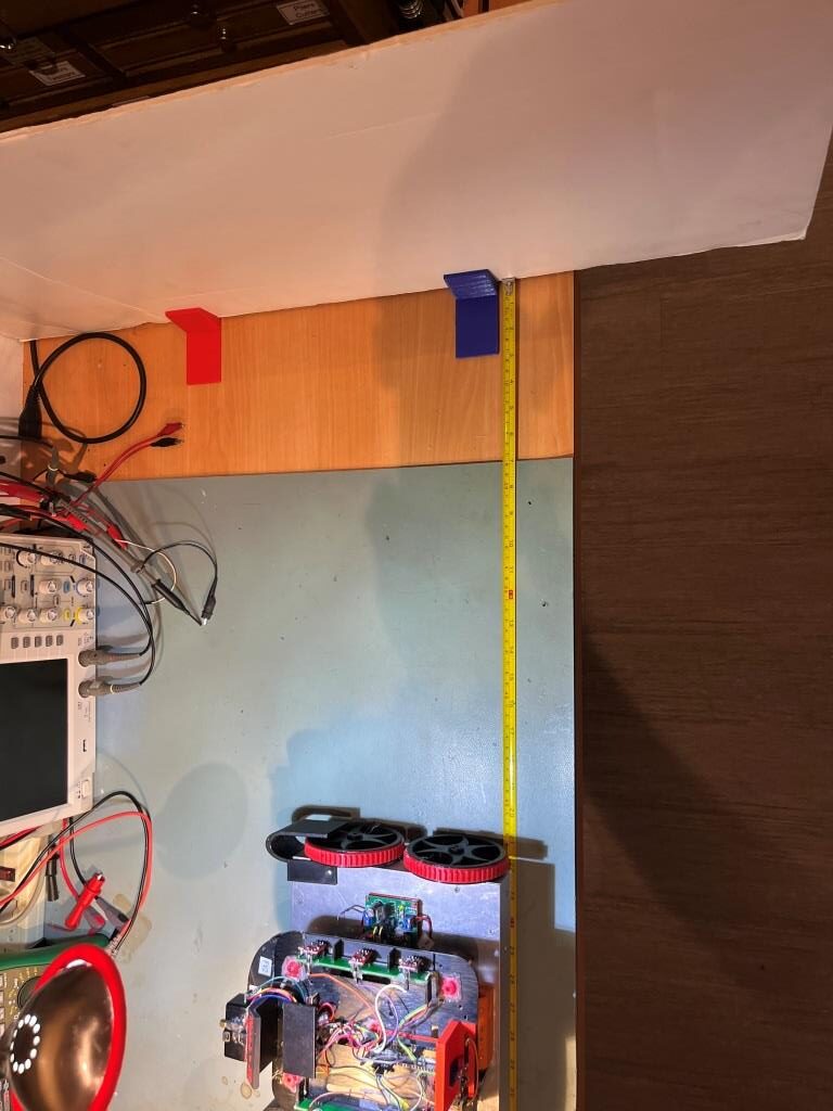
I captured the distance readings from all seven sensors at 10cm intervals from 10 to 60cm, using ‘WallE3_Complete_V2.ino’ in ‘Distances Only’ mode. For each reading I recorded a 20-point average as shown in the following table and plot:
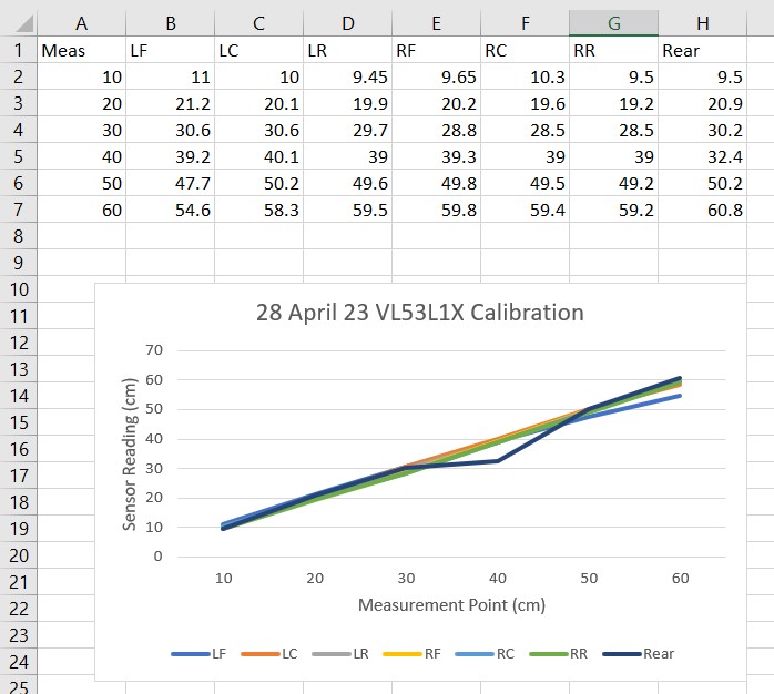
This data looks exceptionally good except for the recorded values for the rear sensor. It looks like I may have made a mistake on the 40cm measurement. To investigate this, I re-ran just the rear sensor measurements, resulting in the following table and plot:
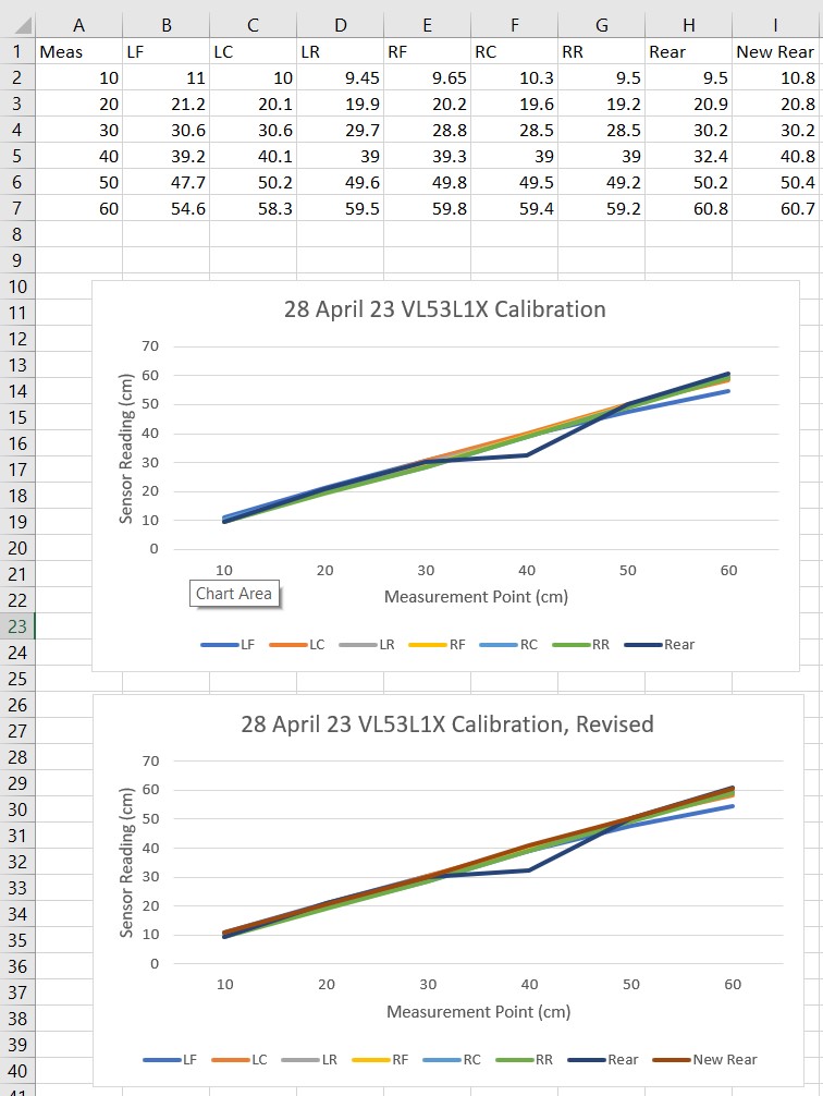
Looking at the data I suspect I simply forgot to move the robot to the new distance for the 40cm ‘rear’ measurement. I dropped the faulty dataset and then used Excel’s ‘trendline’ feature to show a linear expression fit to the data for each sensor, as shown below:
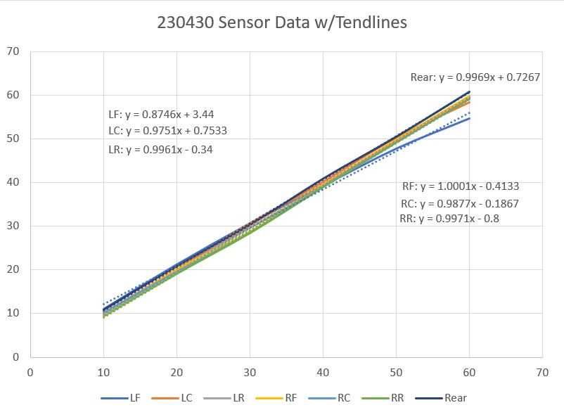
It turned out to be pretty difficult to select individual sensor plot lines to add trendlines, because (with the exception of the left front sensor) they were all almost identical. In order to add trendlines, I had to use Excel’s ‘Select Data’ feature to show only one line at time. Then when I added the associated trend line, I was able to edit the displayed expression to tag it to the associated sensor, as shown above.
As I did in my previous work with the VL53L0X sensors, I used the trendline expressions to come up with compensation expressions for each sensor, as follows:
- LF: LFCorr = (LF-3.44)/0.8746
- LC: LCCorr = (LC-0.7533)/0.9751
- LR: LRCorr = (LR+0.34)/0.9961
- RF: RFCorr = (RF+0.4133)/1.0001
- RC: RCCorr = (RC+0.1867)/0.9877
- RR: RRCorr = (RR+0.8)/0.9971
- Rear: RearCorr = (Rear-0.7267)/0.9969
When I plotted the corrected values, I got the following plot:
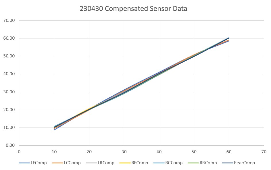
As can be seen in the above plot, the compensation is almost perfect (for that matter, most of the sensors, with the exception of the LF (Left-Front) sensor, were pretty much spot on without compensation.
With the above information, I modified all seven ‘lidar_XX_Correction()’ functions in ‘Teensy_7VL53L1X_I2C_Slave_V1.ino’ to use the new correction factors, and then made another distance measurement run, with the results shown below:
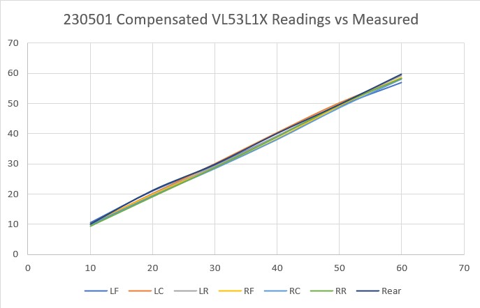
At this point I believe it is time to declare victory and move on with WallE3 ‘field testing’.
Stay tuned,
Frank