Posted 08/15/15

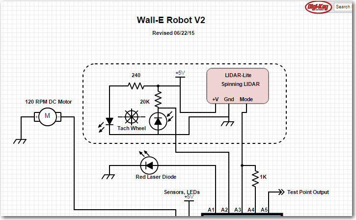
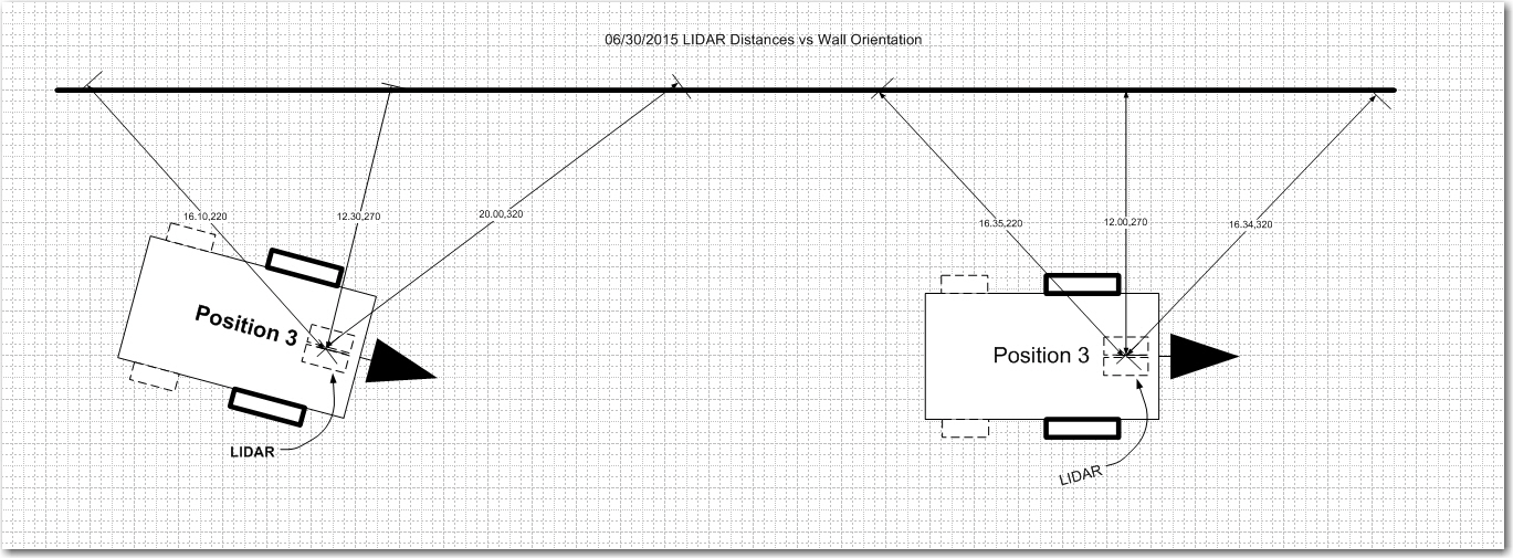
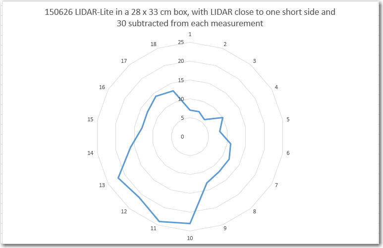
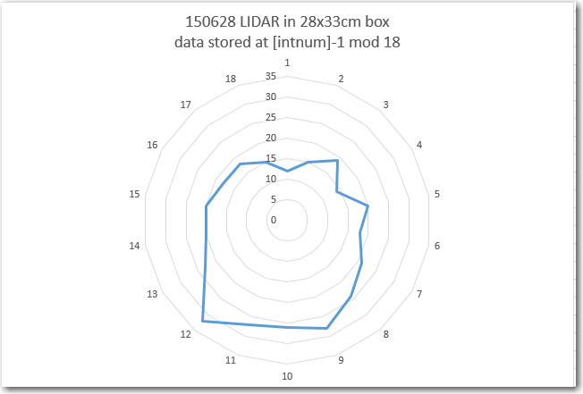
In my ongoing Sisyphean  effort to get Wall-E (my wall-following robot) to actually follow walls, I recently replaced the original three (actually four at one point)  acoustic distance sensors  with a spinning-LIDAR system using the Pulsed Light LIDAR-Lite unit.  While this effort was a LOT of fun, and allowed me to also get some good use from my 3D printers, I wasn’t able to reach the goal of improving Wall-E’s wall-following performance.  In fact, wall-following performance was much WORSE – not better.  As described in previous posts, I finally tracked the problem down to too-slow response from the LIDAR unit – it couldn’t keep up with the interrupts from my 10-tooth tach sensor that provides then necessary LIDAR pointing-angle information.  I tried changing the LIDAR over from MODE control to I2C control (see previous posts), but this led to other issues as described, and although I saw some glimmers of success, I’m still not there.

So, when I noticed that Pulsed Light was advertising their new ‘Blue Label’ (V2) version of their LIDAR-Lite unit, with a nominal 5x response time speedup, I immediately ordered one, thinking that was the solution to all my problems.  A 5x speedup should easily be fast enough to enable servicing interrupts at the 25-30 msec time frame required for my spinning LIDAR setup.  I would be home FREE! ;-).

Well, as it turns out, I wasn’t quite home free after all.  As often happens, the reality is a bit more complicated than that.  When I first received my V2 ‘Blue Lable’ unit and made some initial tests, I immediately started having ‘lockup’ problems of one sort or another, even using the Arduino example sketches provided by Pulsed Light, and with a  470 uF BAC   (big-assed capacitor) installed (Pulsed Light operating recommended 680 uF, but 470 was the biggest I had readily available).

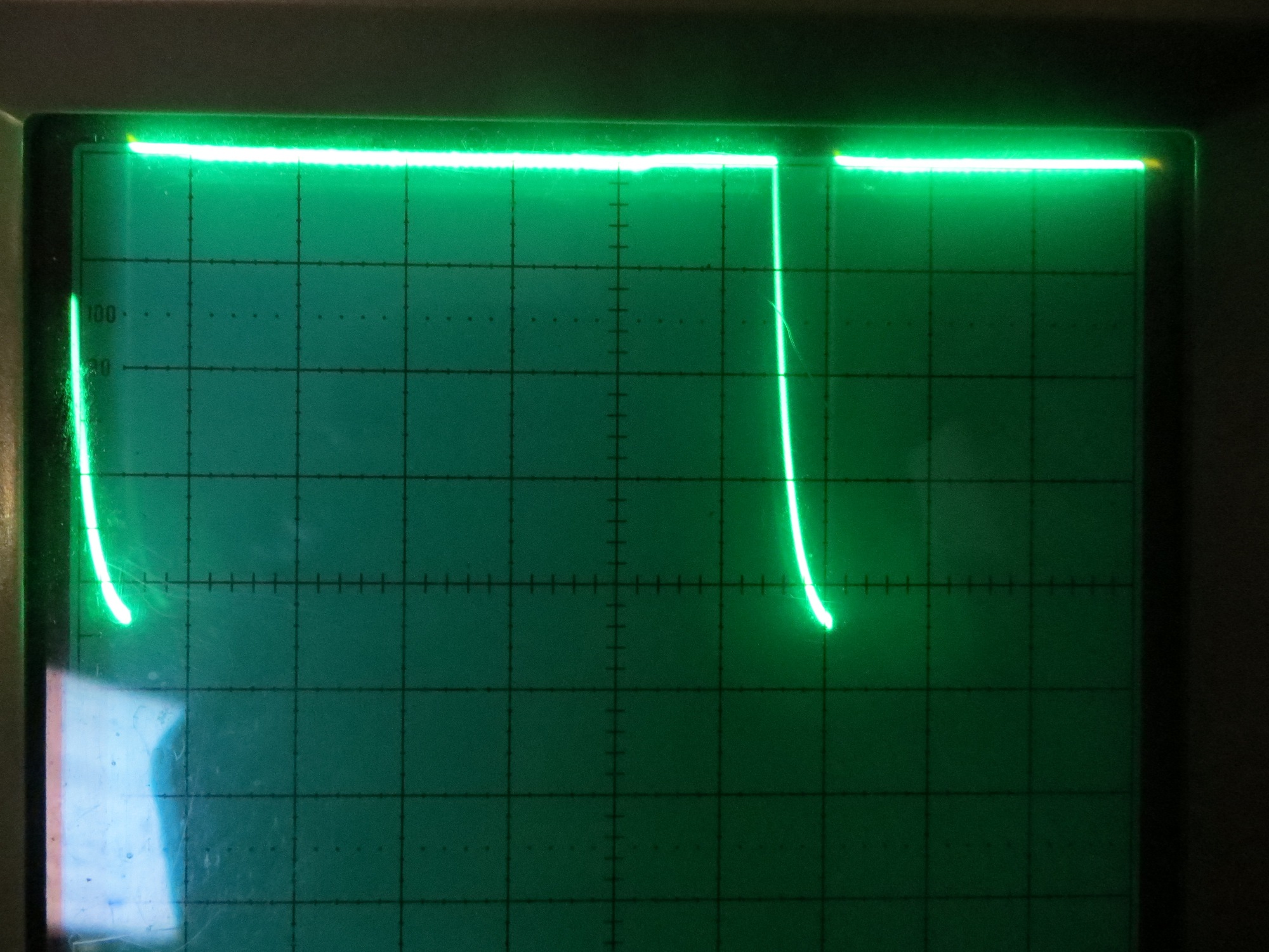
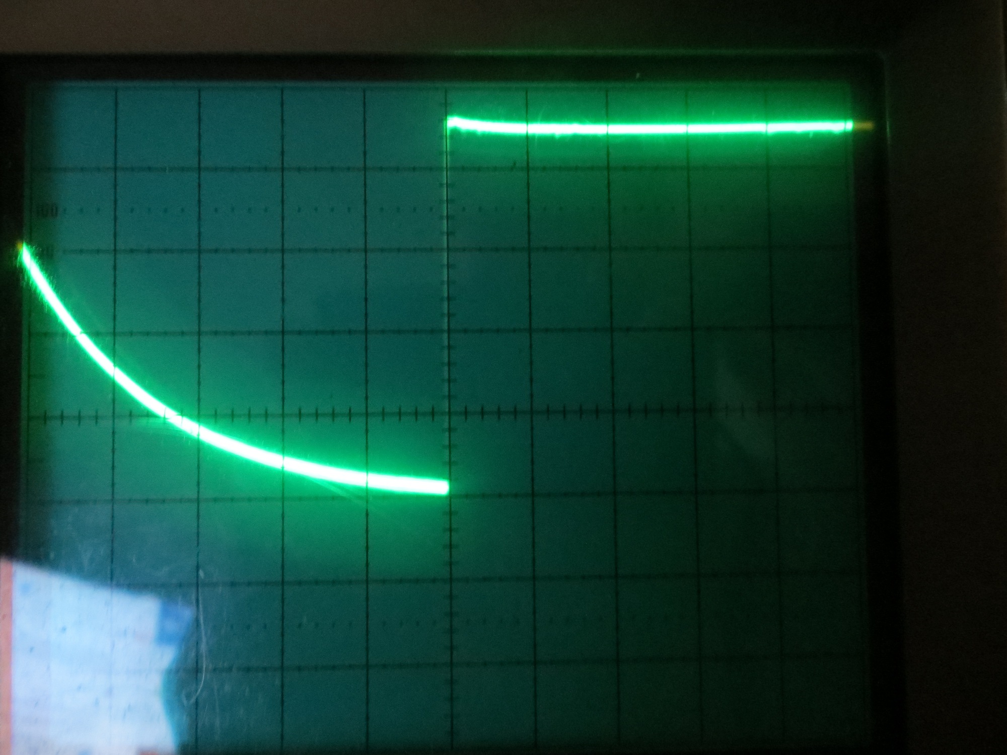
The Pulsed Light supplied ‘Distance as fast as Possible’ Arduino sketch makes a single call to the V2 measurement routine with ‘stabilization’ enabled, and then makes another 99 calls to the routine with ‘stabilization’ disabled. The idea is that the extra time required for the stabilization process is only necessary every 100 measurement or so.  The provided test sketch implements a Serial.println() statement for every measurement, but this can quickly overload the serial port and/or PC buffers.  So, I modified the sketch to print the results of the single ‘stabilized’ measurement plus only the last (of 99) ‘unstabilized’ measurements.  This seemed to work *much* better, but then I noticed that the ‘stabilized’ measurement was showing occasional ‘drop-outs’ where the measurement to a constant 60cm distant target was 1 cm instead of 60 cm – strange.

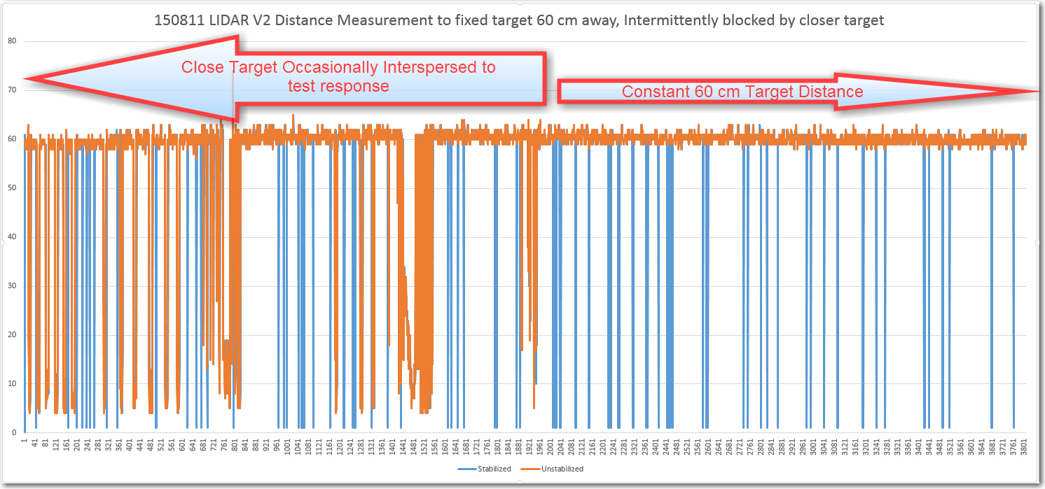
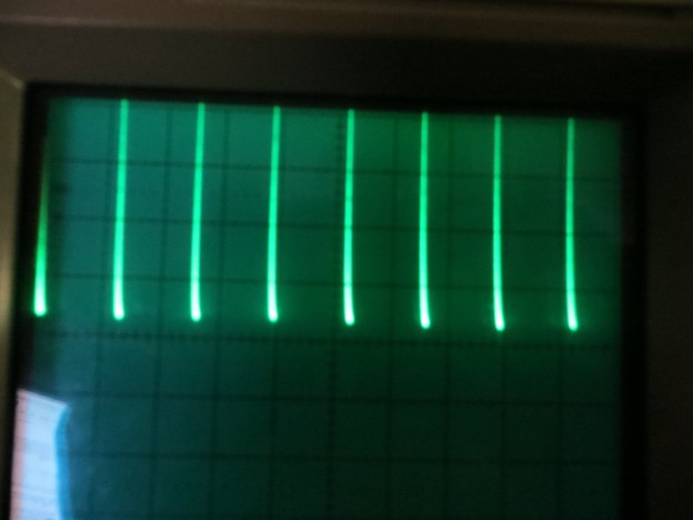
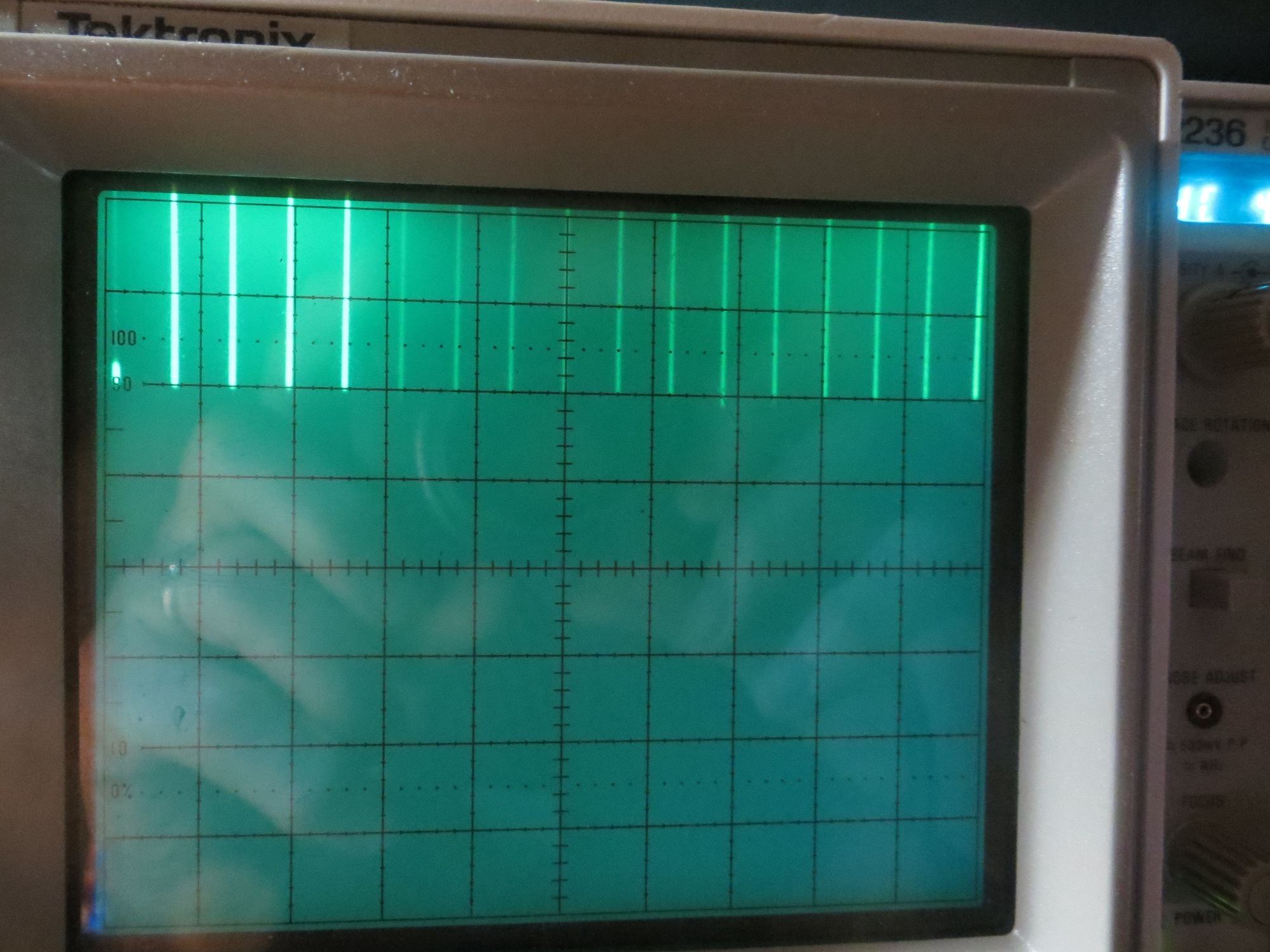
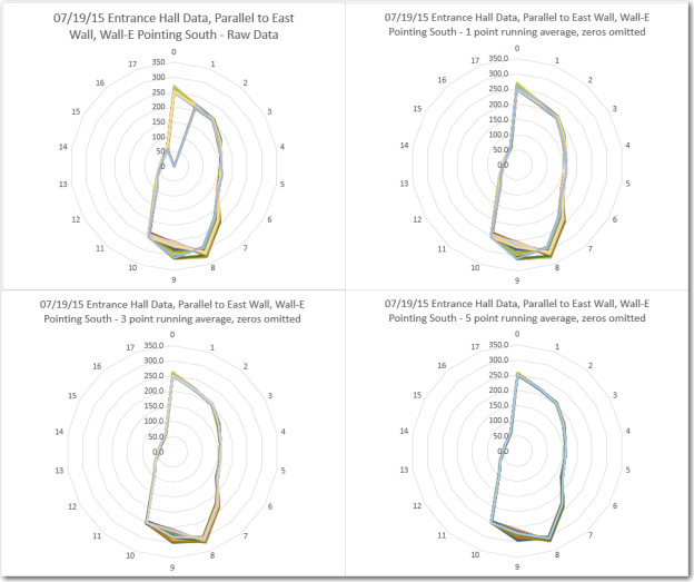
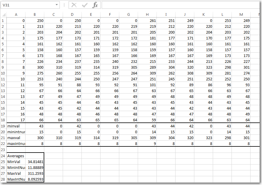
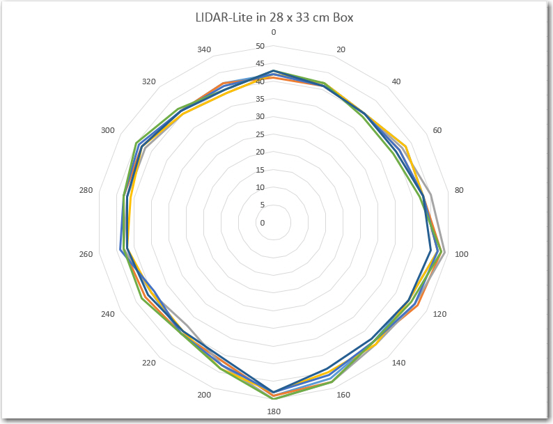
08/11/15 Test with ‘Blue Label’ LIDAR-Lite. Target is a constant 60cm away.

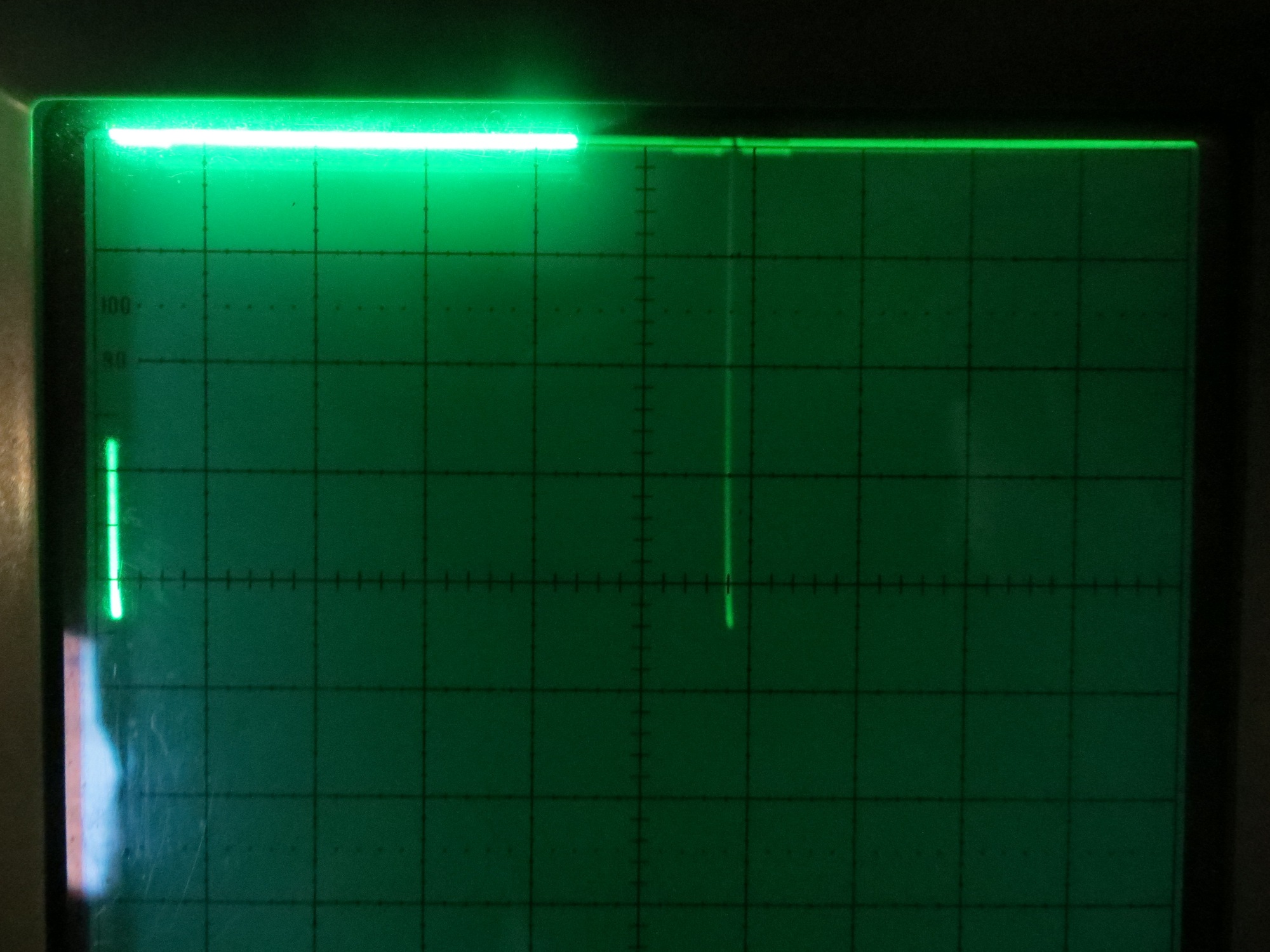
I passed this all along to the Pulsed Light folks (Austin and Bob, who have been very responsive the entire time).  They suggested that the smaller cap might be the problem,  so I ordered replacements from DigiKey.  When they arrived, I ran the same test again, but this time I not only had the ‘stabilized measurement dropout’ problem, but now the unit was consistently hanging up after a few minutes as well.  More conversation with Austin/Bob indicated that I should try using an external power supply for the Arduino rather than depending on the USB port to supply the necessary current.  So, I made up a power cable so I could run the Uno from my lab power supply and tried again, with basically the same result.  The V2 unit will run normally for a while (with ‘stabilization drop-outs’ as before) and then at some point will go ‘ga-ga’ and start supplying obviously erroneous results, followed at some point by a complete lack of response that requires a power recycle to regain control.

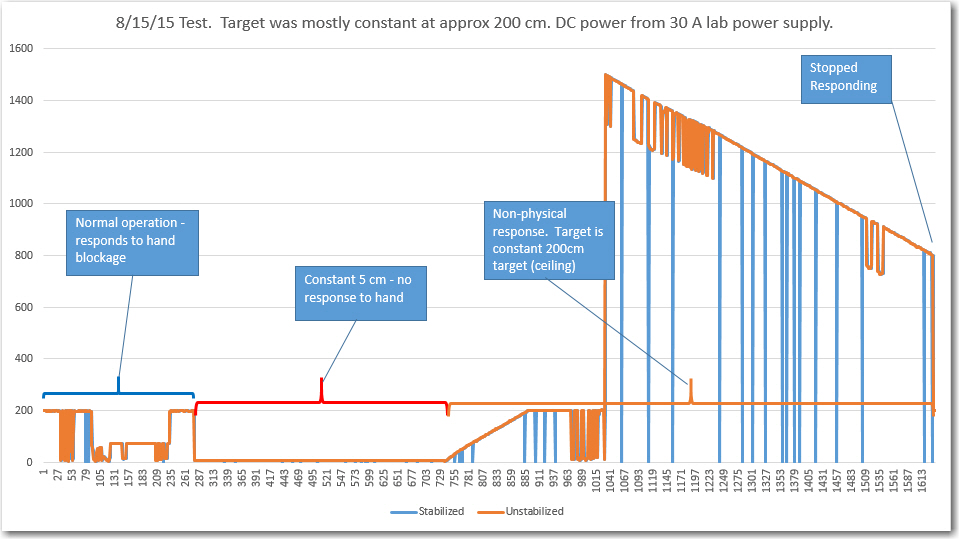
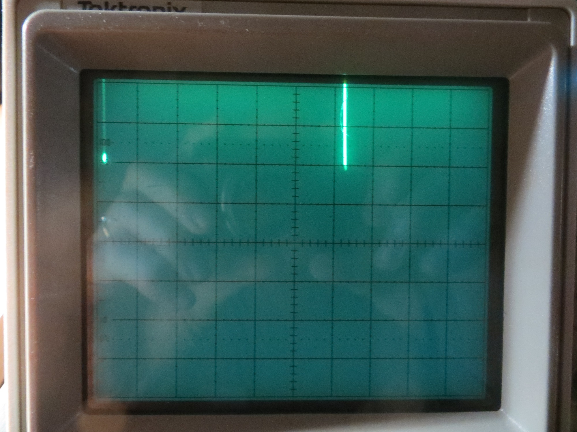
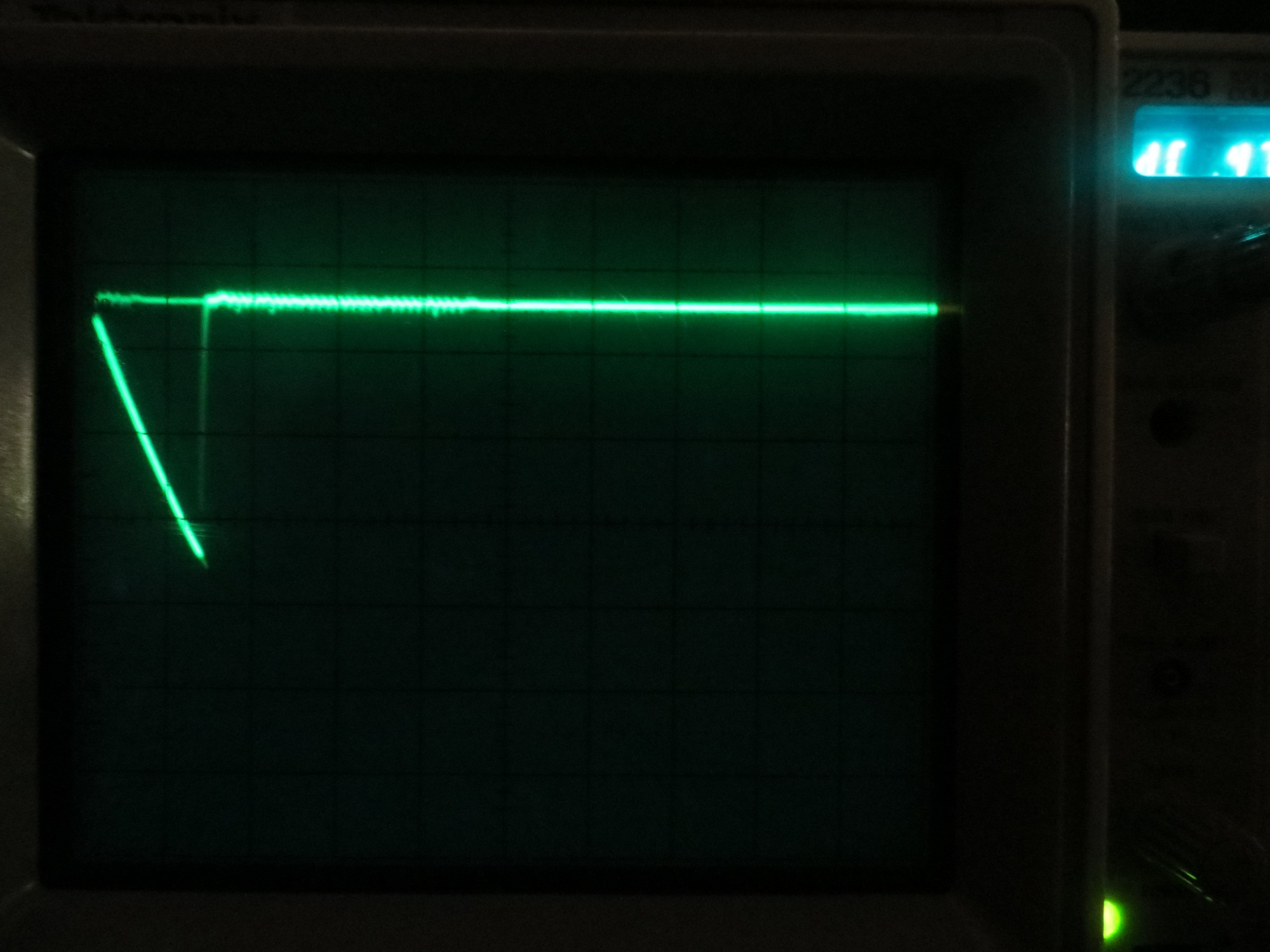
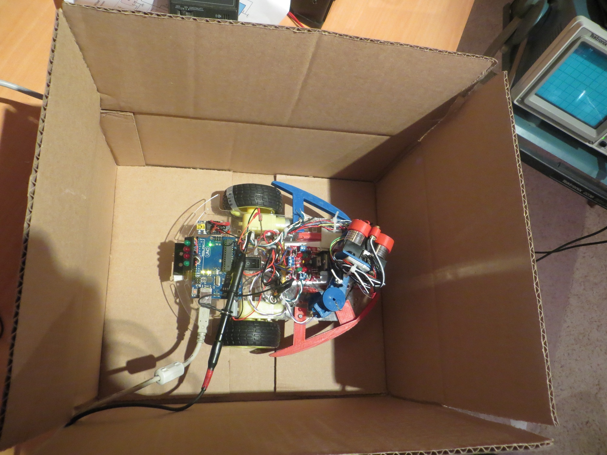
08/15/15 Test with external power supply for Arduino Uno

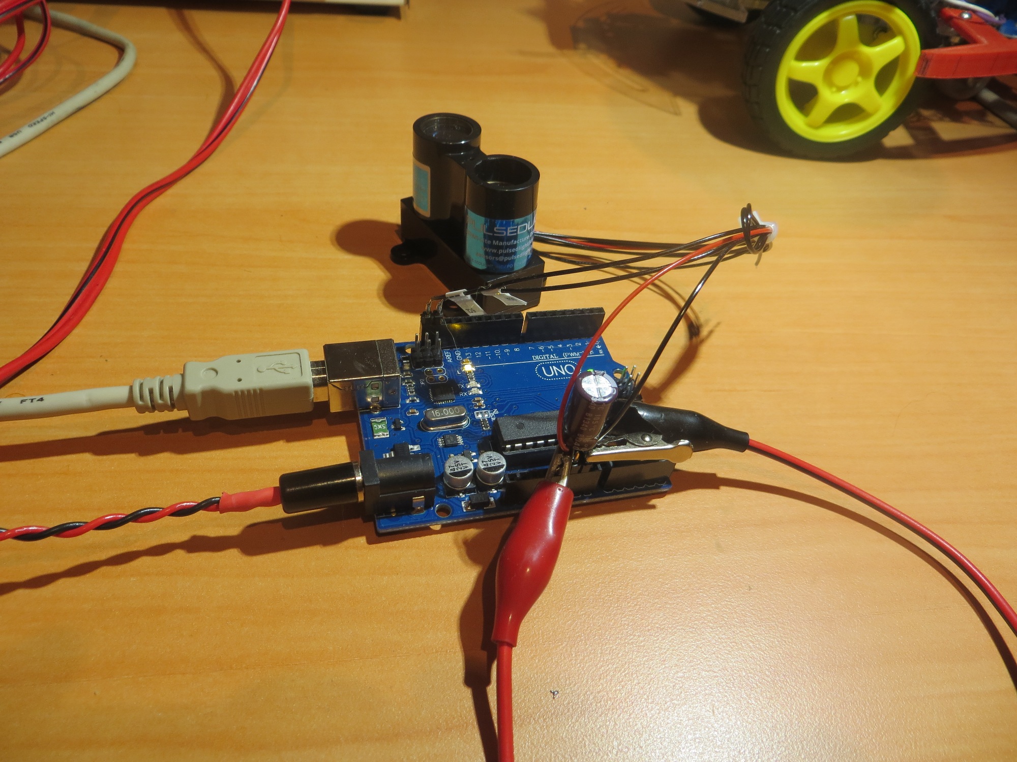
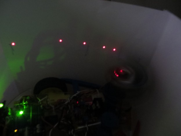
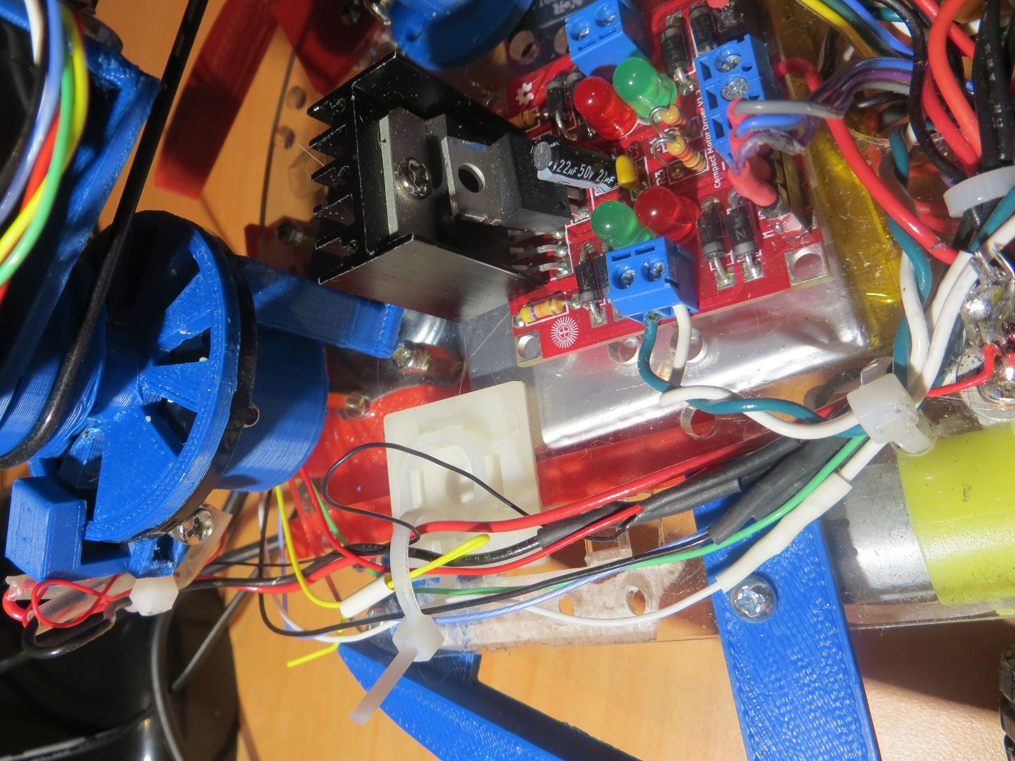
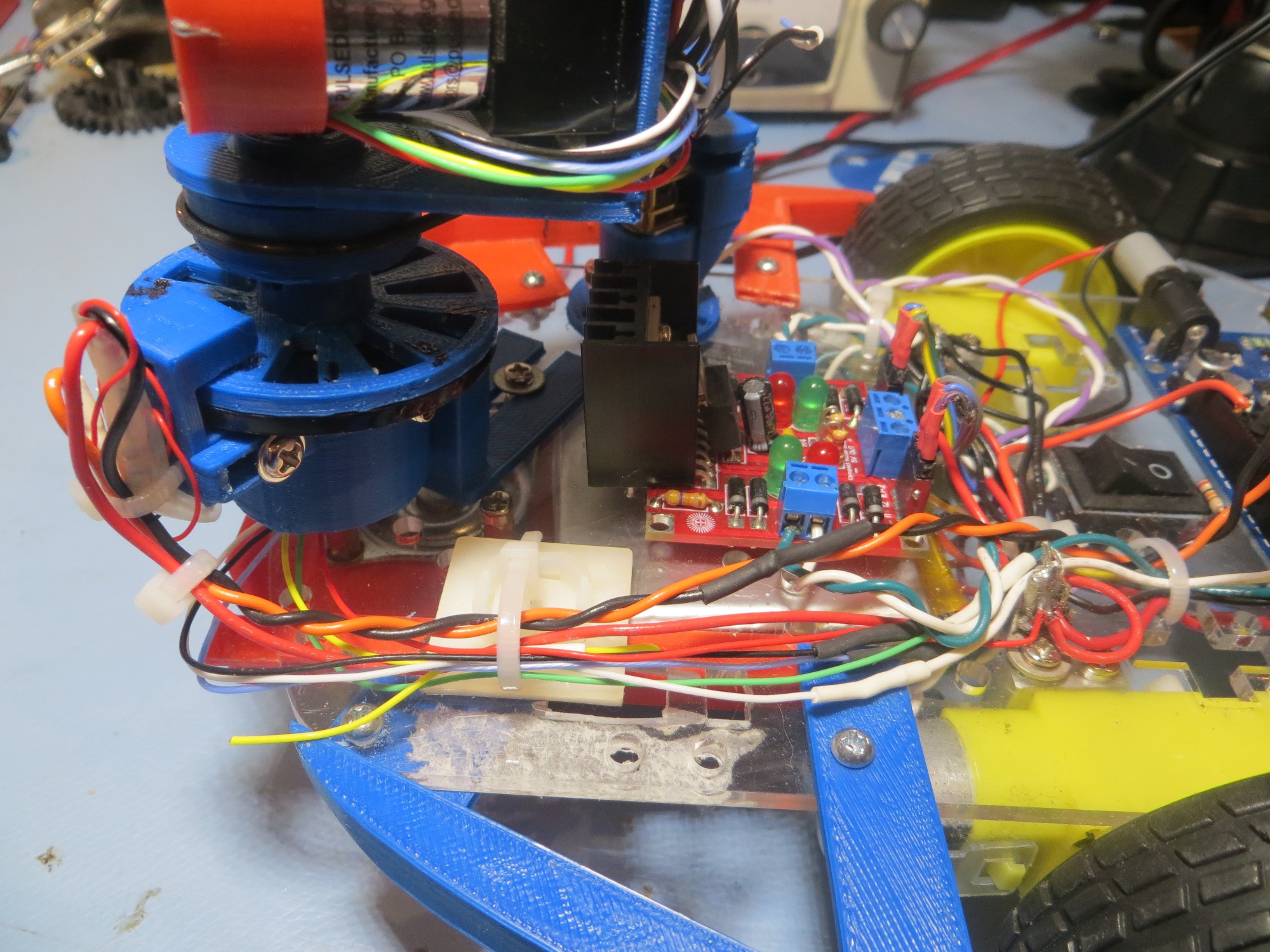
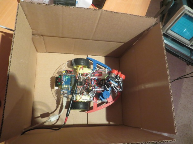
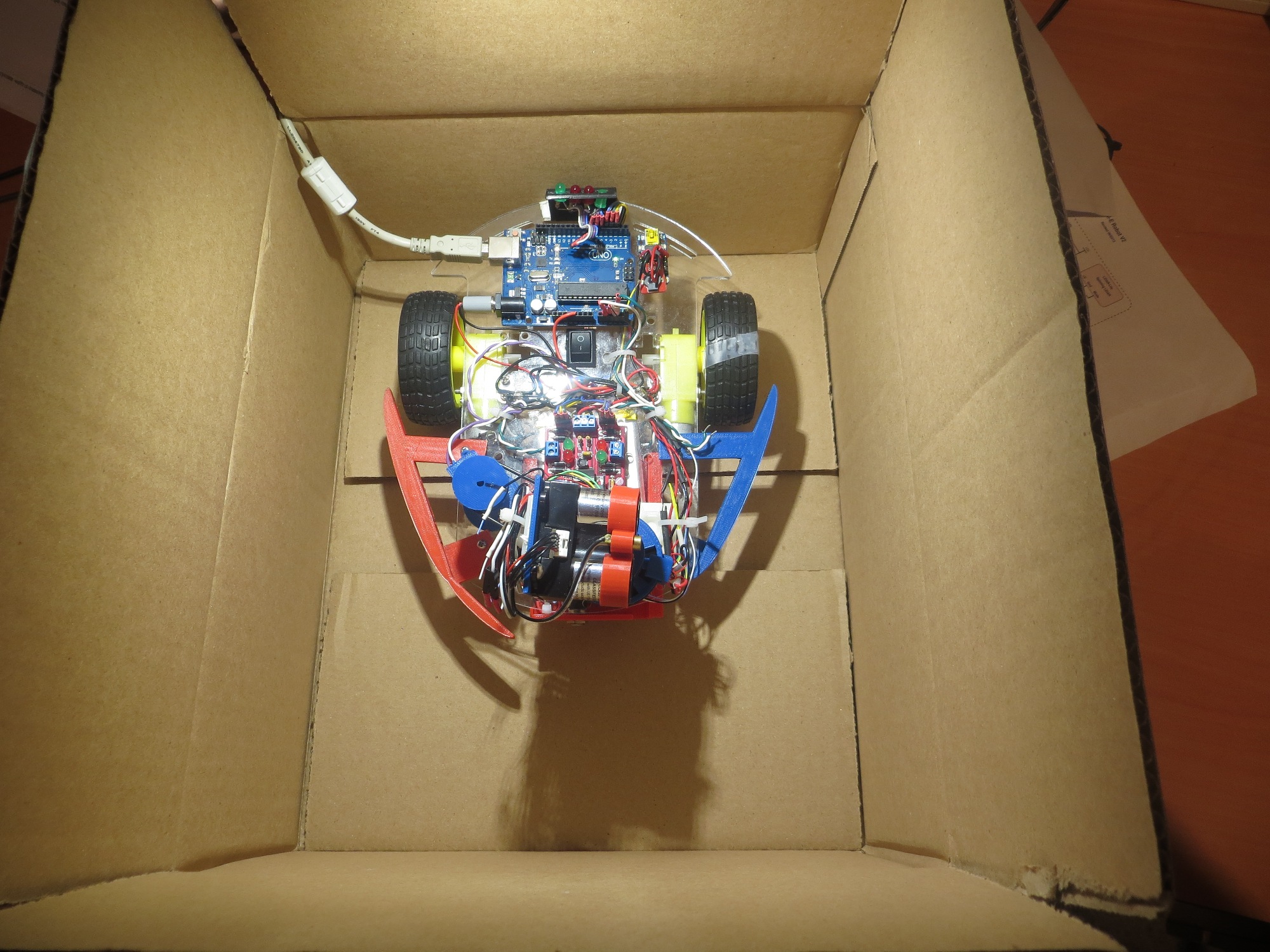
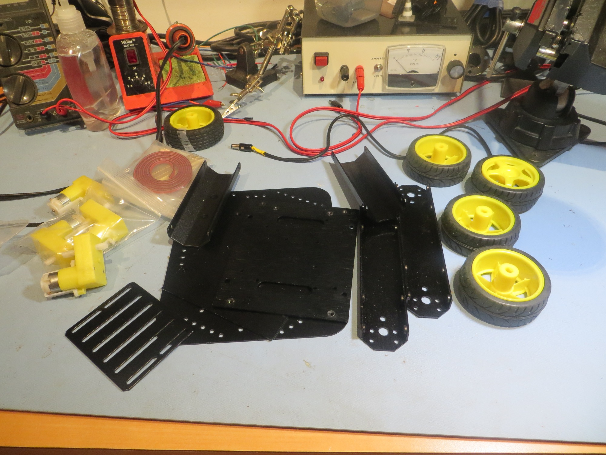
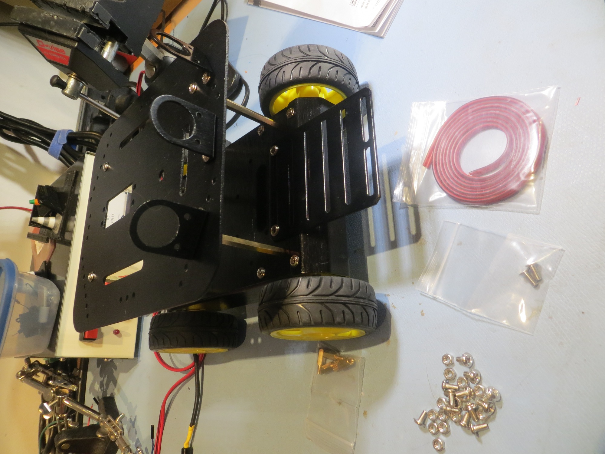
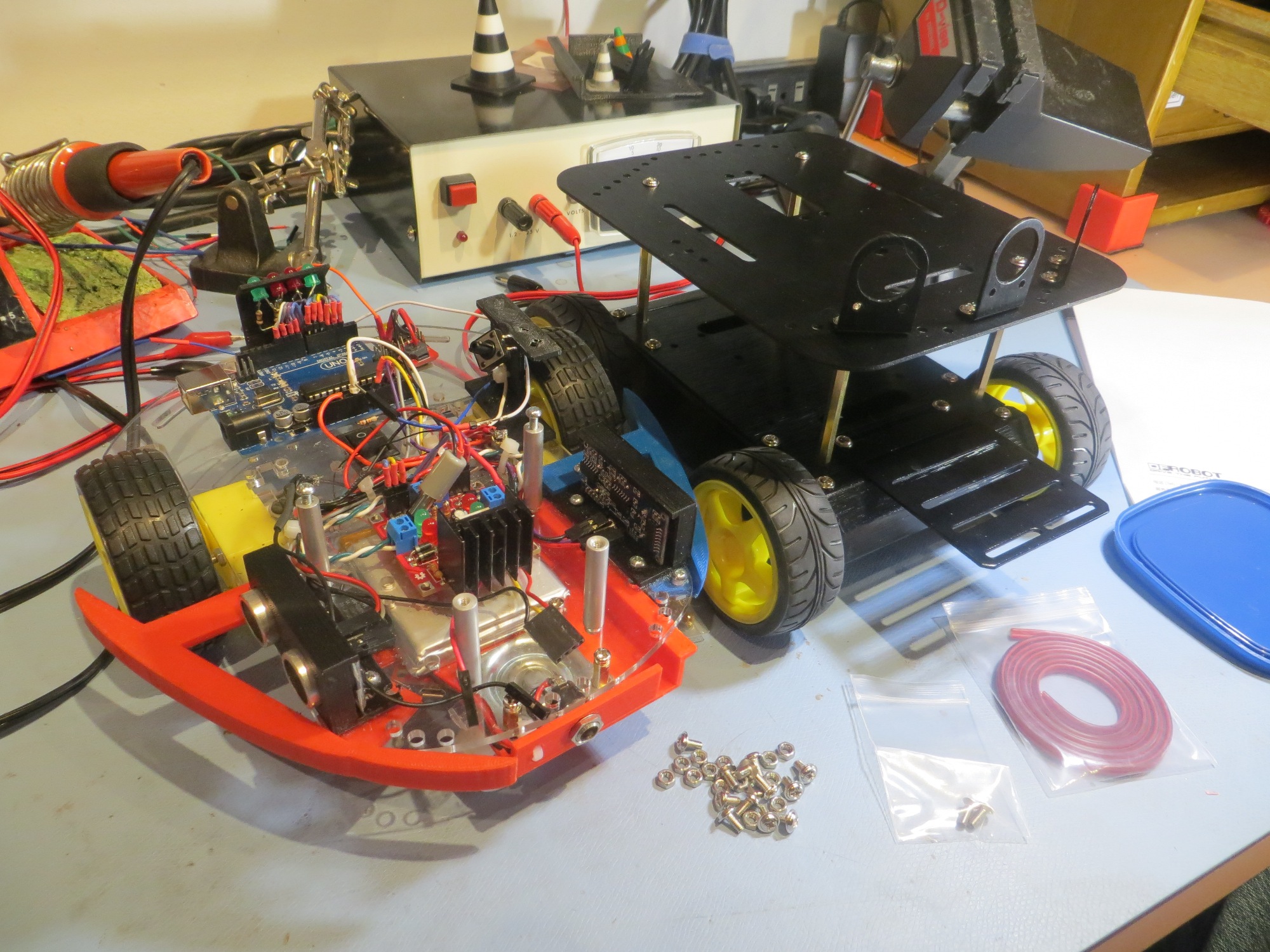
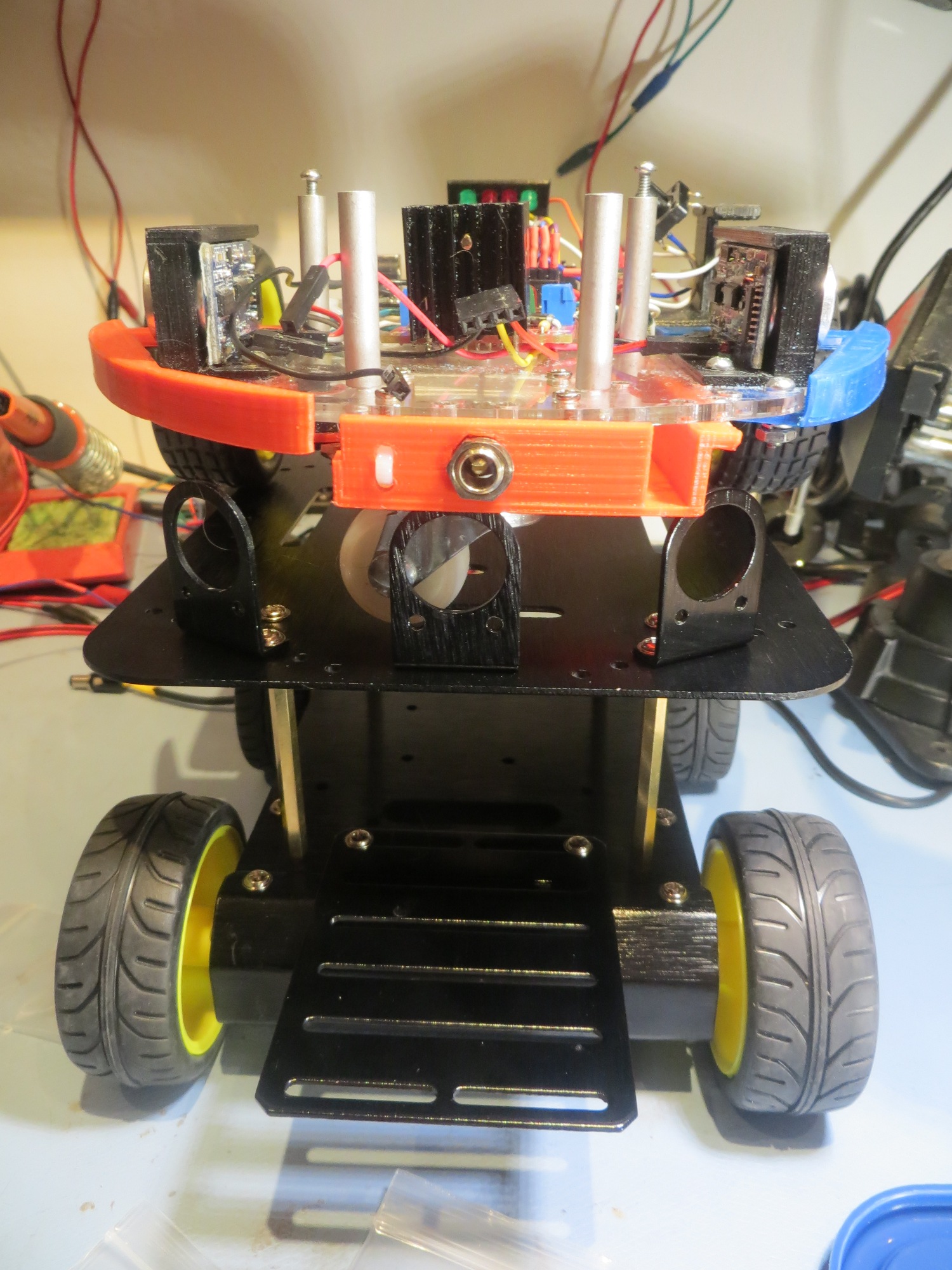
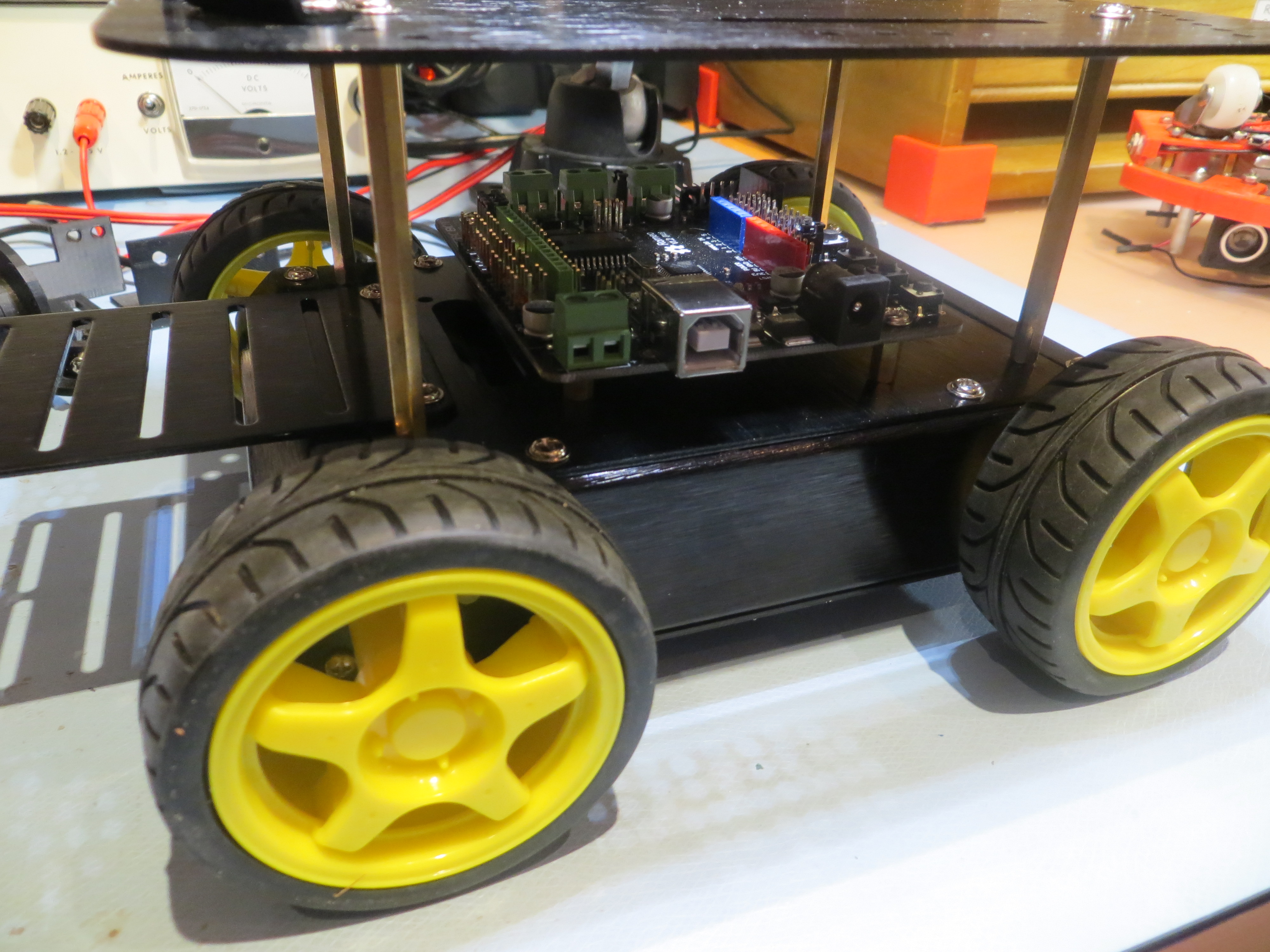
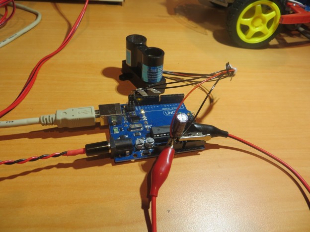
V2 ‘Blue Label’ test setup showing BAC (Big-Assed Capacitor) and external power supply connection

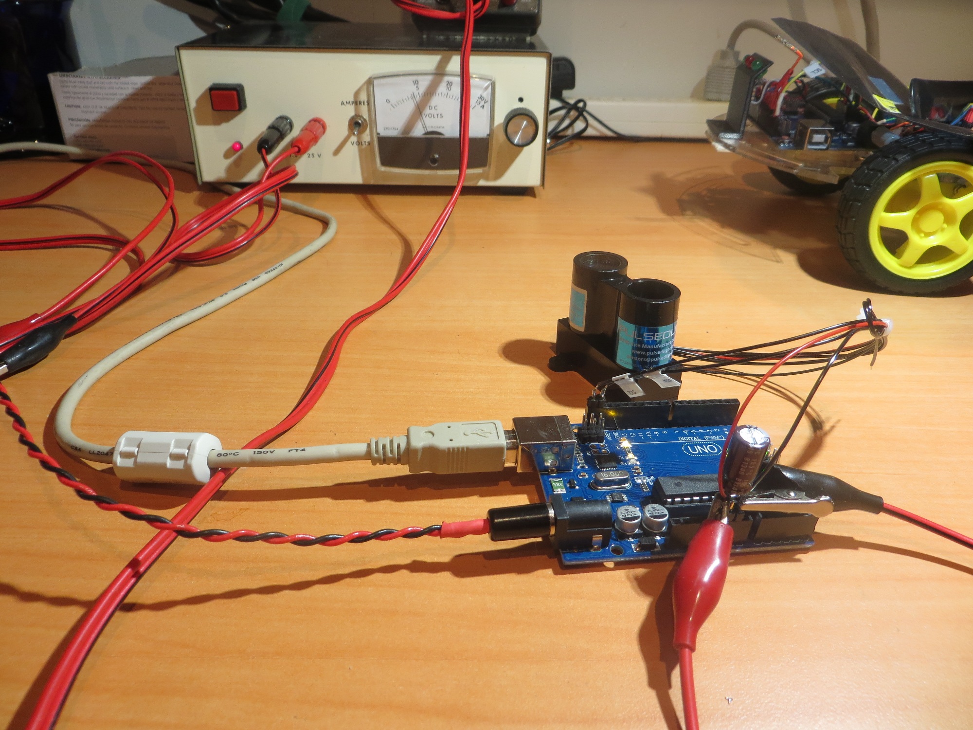
V2 ‘Blue Label’ test setup showing BAC (Big-Assed Capacitor) and external power supply connection

All this went back to Austin/Bob for them to cogitate on, and hopefully they will be able to point out what I’m doing wrong.  In the meantime, I have ordered a couple of ‘Genuine’ Arduino Uno boards to guard against the possibility that all these problems are being caused by some deficiency associated with clone Uno’s that won’t be present in ‘genuine’ ones.  A guy can hope, anyways! ;-).

Stay Tuned!

Frank

Posted 08/12/15

In my last post (http://gfpbridge.com/2015/08/wall-e-has-more-interrupt-issues/) I found that the Pulsed Light LIDAR-Lite (now called ‘V1’ as there is a new ‘Blue Label’ V2 version out) couldn’t keep up with the pace of hardware interrupts from my 10-tooth tach wheel running at about 120 RPM.  So, I decided to try my luck with the I2C interface, as that was rumored to be somewhat faster than the MODE line interface.  I had resisted doing this as it requires the use of the I2C (or ‘Wire’) library, and I thought it would be more trouble to implement.  As it turned out, I was mostly wrong (again) :-).

In any case, changing over from the MODE interface to the I2C interface turned out to be a non-issue.  Pulsed Light has some nice Arduino example code on GitHub, along with clear instructions on what I2C library to use (there are several). I did have to swap out the MODE  line for one of the two I2C lines due to the limitation of 6 wires through the spinning LIDAR slip-ring setup (4 were  already occupied by power, ground, and the two laser diode wires).  However there was some good news in that this freed up one of the Uno’s  analog ports, as the I2C SCL and SDA lines have dedicated pin-outs on the Uno.

Anyway, I got the SCL/SDA lines connected through the slip-ring and to the Uno,  downloaded/installed the necessary I2C library, downloaded and installed the Arduino example, code, and uploaded it to my Uno system.  Sure enough, the example code worked great, and in addition gave much more accurate distance results than with the MODE method (with the MODE method, I had to subtract 40 cm from each measurement.  With the I2C method, the measurements seemed to be ‘dead on’).

However, when I instrumented the code to toggle a Uno digital pin so I could measure the timing with my trusty O’Scope, I received a major shock.  Instead of the 30-35 msec cycle time from the MODE method, the I2C method was showing more like 110-120 msec – MUCH slower than the MODE method, and WAY too slow for servicing interrupts at 20-25 msec intervals!

Yikes – what to do?  Well, as usual when I’m faced with a situation I don’t understand, my response is to yell for help, and  take more data.  the ‘yell for help’ part was accomplished via an email to ‘help@pulsedlight3d.com’, and the ‘take more data’ part is described below.

The first thing I did was to  re-download the Pulsed-Light test code from GitHub and run it again without any modifications.  The test program simply writes distances out to the PC console, and I was able to re-verify that the LIDAR unit was indeed responding with what appeared to be correct distances, and responded appropriately when I waved my hand in front of the optics.

Next, I added a line of code at the top of the test code’s Loop() section to force the Uno’s LED pin (pin 13) HIGH, and another one at the ‘bottom’ (after the measurement but before the Serial.println() statement) to force the LED pin LOW.  This gives me the ability to directly view the measurement timing on my trusty O’Scope.  The reason the LOW statement line has to be before the Serial.println() statement is that the bottom of the Loop() code and the top are actually the same point in time, which would effectively put the HIGH and LOW statements right next to each other, making O’Scope measurements impossible.  By putting the LOW statement before the Serial.println() statement, I am guaranteed to have a LOW period equal to the time it takes the Serial.println() statement to convert the distance value to a string and send it to the serial port.

After uploading the above modification to the Uno, I got the following Scope screenshots:

20msec/div showing the ’20msec’ mode.

20msec/div showing the ‘100msec’ mode, where the LOW between measurement pulses are spaced approximately 100 msec apart.

0.1 msec/div closeup of the LOW period between the ‘bottom’ and ‘top’ of the Loop() section. Note the curved section at the bottom is due to the LED turning OFF.

The first image above at 20msec/div shows what I expected to find – that the LIDAR-Lite V1 unit is capable of taking measurements with  an approximate 20msec cycle time.  This  should work fine for my Wall-E spinning LIDAR  robot, as interrupts from the tach wheel sensor occur at about 25msec intervals.

However, after a few minutes, the scope display (again at 20msec/div) showed that the system stopped responding a the 20msec rate, and instead started responding no faster than about 100-110msec, WAY too slow for my spinning LIDAR application.  I have no idea why this happens, but I am hoping the Pulsed Light guys will tell me that I have simply screwed something up and doing XYZ will fix it.

The last image above  at 0.1msec/div shows a closeup of the OFF period.  The curved bottom section is due to the fact that the LED turns OFF at about 3 Vdc, and below that the remaining energy has to be drained off through a high impedance.

After sending this information off to the PL guys, I started thinking that maybe the apparent change from ’20msec’ mode to ‘100msec’ mode  might  possibly be due to the extremely short LOW duration (about 100 usec or less) and the fact that the LOW doesn’t go much below about 3Vdc.  Although I didn’t really believe it, I thought it was just barely possible that my trusty O’Scope was just missing these very short transitions after a time, and the whole problem was an O’Scope problem and not a LIDAR problem.  So, in order to put this possibility to rest, I modified the code again to extend the LOW duration by 1msec with a delay(1) statement just after the line that sets the LED output LOW (essentially adding an extra 1msec delay between the LOW and HIGH lines).  After uploading this to the Uno, I captured the following O’Scope waveforms.

After addition of a 1msec delay to the LOW period. Showing the ’20msec’ mode at 10msec/div

After addition of a 1msec delay to the LOW period. 2msec/div

After addition of a 1msec delay to the LOW period. 0.2 msec/div closeup of the LOW period between the ‘bottom’ and ‘top’ of the Loop() section. Note the curved section at the bottom is due to the LED turning OFF.

After addition of a 1msec delay to the LOW period. This shot was taken about 45 minutes after startup, showing that the system has made an uncommanded transitioned to ‘100msec’ mode

As shown in the above photos, I got essentially the same behavior as before.  The system came up in ’20msec’ mode, but made an uncommanded transition to ‘100msec’ mode about 45 minutes after startup.

So, something is happening here, but I don’t know what it is.   It ‘smells’ like a heat-related problem, but that doesn’t make a whole lot of sense, as I’m running this in an air-conditioned environment, and there isn’t that much power being used as it is.  As I mentioned above, I’m hoping it’s just something dumb that I’m doing that is causing this, but I have no clue what that might be.

There is one other possibility that just popped into my head.  I’m using Uno clones rather than actual Arduino boards.  I guess it is just barely possible that the problem is in the Uno board, not the LIDAR. Maybe the I2C lines get flaky after some time, and start sending bad requests to the LIDAR or not properly processing LIDAR responses?  I’m thinking I might want need to  acquire some genuine (Genuino?)  Arduino Uno boards to eliminate this possibility.

Stay tuned!

Frank

Posted 08/04/2015

In my last post (http://gfpbridge.com/2015/07/emi-problems-with-lidar-and-wall-e/) I described my efforts to track down and suppress an apparent EMI problem with Wall-E. After successfully (I hope) killing off the EMI problem, I added navigation code back into the mix, and did some initial tracking tests on  a long, straight wall.   The results were not encouraging at all – it appeared that Wall-E was having quite a bit of difficulty deciding which way to steer; it appeared to be correctly measuring the distance and angle to the nearest obstacle (the wall), but wasn’t adjusting wheel speed to compensate for nose-in or nose-out conditions.

As it turned out, there was a very obvious reason Wall-E wasn’t adjusting the wheel speeds; at some point I had overridden the wheel speed setting logic and arbitrarily pegged the wheel speeds at 50 and 50 – oops!  Unfortunately, while I was figuring this out, I discovered something even more disturbing.  Apparently, all this time Wall-E has been servicing only about half (9 vs 18) of the LIDAR tach wheel interrupts!  I hadn’t noticed this up until now because although I had previously looked at the the contents of the 18-element distance/time/angle array, there was apparently enough ‘creep’ in the interrupt numbers that Wall-E *did* service that the array looked normal.  However, some of the instrumentation code I put in place this time made it painfully obvious that only 9 interrupt calls were being made.  As a double-check, I changed the code to turn the red laser ON during interrupt service routine (ISR) calls, and OFF at all other times.  Then I made a surround screen from several sheets of paper and looked at the pattern made by the laser.  In the following time-lapse image (0.5 sec or about 1 full revolution), 4 laser pulses (ISR calls) are visible in about 1/2 full circle.  In the following video, there are only 9 laser pulses visible  per revolution.

Time Lapse (0.5 sec) photo with GetMeasure() call in

Then I went into the code, and commented out the call to GetMeasurement().  GetMeasurement() is where the Pulsed Light LIDAR measurement delay occurs, and  this is the obvious suspect  for missing ISR calls.  As the following time-lapse photo and companion video shows, this indeed allowed all 18 ISR calls per revolution.   Comparing the two photos, it is obvious that the one without the GetMeasurement() call exhibits twice as many laser pulses (ISR calls) and each pulse is much shorter, denoting less time spent in the ISR.

Time Lapse (0.5 sec) photo with GetMeasure() call commented out.

So, what to do?  In the first place, I’m still not sure  why  interrupts are being skipped.  If you believe that the laser ON time represents the duration of a particular ISR call, then the fact that there are times when the laser is OFF should indicate that the system can service another interrupt – why doesn’t it?

So, back to the drawing board.  I drug out my trusty O’Scope and started poking around.  I have one of the Uno’s digital lines set up to show the duration of GetMeasurement() and another one  set to show the duration of the ISR.  Then I did a series of tests, starting with GetMeasurement() turned ON as normal,  but with the call to PulsedIn() (the actual LIDAR measurement function) commented out and replaced with delays of 10, 20, and 30 msec.  The following captioned photos show the results:

Conclusions:

• The PulseIn() call in GetMeasurement() is definitely the culprit.  Not surprising, as this is the call that interfaces with the spinning LIDAR unit to get the actual distance measurement.  The only question is  how long  does/should it take the LIDAR to return the distance measurement.
• Delays up to 20 msec in place of the PulseIn() do not adversely affect operation.  Both the O’Scope and laser pattern presentations clearly show that interrupt servicing is proceeding normally.
• A 30 msec delay is too large, but not by much.  There is some evidence in the O’Scope photo that occasionally the next interrupt  is not skipped.

The above conclusions track reasonably well with the known physics of the setup. The spinning LIDAR rotates about 2 times/sec, or about 500 msec/rev.  Interrupts are spaced out 1/20 rev apart, except for the index plug where 2 interrupts are missing.  (500 msec/rev)  times  (1/20 rev/interrupt) = 25 msec/interrupt.  So, 10msec delay should be no problem, 20 should also fit, but 30 is too long.  The fact that there is some evidence that 30 is almost short enough is probably due to the rotation speed being slower than estimated; 30 msec/interrupt –> 600msec/rev or about 20% slower than nominal.

In any case, it is clear that the current setup can’t support an interrupt interval of 25 msec.  I’m either going to have to slow down the spinning LIDAR (which I do not want to do) or speed up the measurement delay (which I don’t know how to do – yet).

There are two methodologies for interfacing with the Pulsed Light LIDAR.  One (the one I’m using now) is pretty simple but involves the PulseIn() call with it’s known issues.  The other one is via the I2C channel, which I have not tried because I thought would be harder to do, and there wasn’t any real evidence that it was any faster.  Now that I’m convinced that PulseIn() won’t work, I’m going to have to take another look at the I2C interface technique – EEK!!

Stay tuned,

Frank

After getting the Pulsed Light spinning LIDAR system working on Wall-E, I added motor control and navigation code to my LIDAR test code, just to see how if  the LIDAR  could be used for actual navigation.  As it turned out, I discovered two problems; one was related to missed LIDAR distance measurements that got loaded into the nav table as ‘0’s, (see my previous post on this issue) and the other was that interrupts stopped occurring after some indeterminate time after the motors were enabled.  Of course, these glitches just had to occur while my control-systems expert stepson  Ken Frank  and his family were visiting.  I told him about the symptoms, and speculated that maybe noise from the motor control PWM pulse train was coupling into the high-impedance interrupt input  and overloading the interrupt stack with spurious interrupts.  This input is driven by the analog signal from the tach wheel sensor (IR photodiode), and the signal line runs along the same path as one of the motor drive twisted pairs.   Without any hesitation, Ken  said  “well, if you had converted that analog signal to digital at the source, you wouldn’t be having this problem”.  This was absolutely correct, and not a little bit embarrassing, as I distinctly remember teaching  him all about the perils of low-level analog signals in proximity to high-level motor currents!  I guess it’s better to receive one’s comeuppance from a loved family member and fellow EE, but it’s  still embarrassing ;-).

In any case, it’s now time to address the EMI problem.  I’m not absolutely sure that the issue is motor currents coupling into the analog sensor line, but it has all the earmarks; it doesn’t happen unless the motors are engaged, and the sensor line is in close proximity to one of the high-current motor drive  twisted-pairs for some of it’s length.  Moreover, I neglected to follow basic low-level analog handling protocol by using a twisted pair with a dedicated return line for this signal, so at the very least I’m guilty of gross negligence :-(.

Black loop is part of the analog signal run from photodiod sensor on left to Uno (not shown). Note green/white motor drive twisted pair

In the screenshot above, the thin black wire (visible against the white stay-strap mounting square background) is the analog output line from the tach wheel sensor circuit.  This line runs in close proximity to one of the motor drive twisted pairs for an inch or so (extreme right edge of the above image) until it peels off to the right to go to the Arduino Uno.

As shown below,  this circuit has an equivalent output impedance of about 20K ohms (20K resistor in parallel with the reverse bias impedance of the photodiode), so while it’s not exactly a low-level high-impedance output, it’s not far from it either.  The black wire in the photo is the connection from the junction of the 20K resistor and the photodiode to pin A2 of the Uno.

Although I have looked at the A2 input pin with an Oscilloscope (my trusty Tektronix 2236) and didn’t see anything that might trigger spurious interrupts, it doesn’t have the bandwidth to see really fast transitions.  And, as I was once told many many years ago in the TTL days, “TTL circuits can generate  and respond to sub-nanosecond signals”.  Although TTL has gone the way of the dinosaurs (and old engineers like me), the old saw is still applicable.

Portion of Digikey Scheme-It schematic showing tach sensor circuit

So, what to do?  Well, the obvious starting place is to replace the single wire signal run with a twisted pair, adding a dedicated return wire.  In the past, just replacing a single line with an appropriately terminated twisted pair has shown to be remarkably effective in reducing EMI coupling problems, so I’m hoping that’s all I have to do.  The following photo shows the modification

Single black tach sensor wire replaced with orange/black twisted pair

In the above photo, the orange/black twisted pair replaced the single-line tach wheel sensor signal line.  The orange wire is the signal wire and the black wire is the dedicated return line.  The return line is routed to a nearby ground pin on the Arduino Uno.  As an additional precaution, I installed  a 0.01  Î¼F cap between the signal input and the ground pin.

After these modifications, I fired up Wall-E with the motors engaged, and was relieved to find that tach wheel sensor interrupts appear to continue indefinitely, even with the motor drive engaged – yay!!

July 25,  2015

In my last LIDAR-related post (http://gfpbridge.com/2015/07/lidar-field-test-with-eeprom/), I described a test intended to study the question of whether or not I could use LIDAR (specifically the Pulsed Light spinning LIDAR system on Wall-E) to determine Wall-E’s orientation with respect to an adjacent wall, in the hopes that I could replace all the former acoustic sensors (with their inherent mutual interference problems) with one spinning LIDAR system.  In a subsequent field test where I used LIDAR for navigation, Wall-E fared very badly – either running into the closest wall or wandering off into space.  Clearly there was something badly wrong with either the LIDAR data or the algorithm I was using for navigation.

This post describes the results of some follow-on testing to capture and analyze additional LIDAR data from the same hallway environment.   In the last test, I used the Arduino Uno’s EEPROM to store the data, which meant I was severely limited in the amount of data I could capture for each run.  In this test I instead ran the program in DEBUG mode, with ‘Serial.print()’ statements at strategic locations to capture data.  To avoid contaminating the data with my presence, I ran a USB cable out an adjacent door.  I placed Wall-E in about the same place as in the previous post, oriented it parallel to the wall, and started collecting data  after I was safely on the other side of the adjacent door.  I collected about 30 seconds of data (50 or so 18-point datasets) to be analyzed.  The screenshot below shows some of the raw LIDAR data plus a few interesting stats.

Screenshot showing raw LIDAR data with some stats

Looking at the raw data it was immediately clear why Wall-E was having trouble navigating; I was using an algorithm that depended on the stability of the pointing direction (interrupt number) associated with the minimum distance value, and this was unstable to say the least.  The minimum distance value jumped between approximately 43 and 0, and the associated interrupt number jumped between  0 and either 14 or 15.  A  distance value of ‘0’ results from a LIDAR distance measurement failure where the corrected distance is less than zero.  Such values get replaced by ‘0’ before being loaded into the distance/angle array (and subsequently read out to the measurement laptop in this experiment).

So, what to do?  I decided to try some ‘running average’ techniques to see if that would clean up the data and make it more usable for navigation. To do this I wrote up some VBA code to perform an N-point running average on the raw data, and produced results for N = 1, 3, and 5, as shown below.

1-point running average (essentially just zero replacement with the preceding value)

3-point running average, with zero runs longer than 3 replaced with preceding value(s)

5-point running average, with zero runs longer than 5 replaced with preceding value(s)

LIDAR distance ‘radar’ plots of raw, 1, 3, and 5-point running average

Looking at the above results and plots, it is clear that that there is very little difference  between the 1, 3, and 5-point running average results.  In all three cases, the min/max values are very stable, as are the associated interrupt numbers.  So, it appears that all that is needed to significantly improve the data is just ‘zero-removal’.  This should be pretty straight-forward in the current processing code, as all that is required is to  NOT  load a ‘bad’ measurement into the distance/angle table – just let the preceding one stay until a new ‘good’ result for that interrupt number is obtained.  With two complete measurement cycles per second, this will mean that at least 0.5 sec will elapse before another measurement is taken in that direction, but (I think) navigating on slightly outdated information is better than navigating on badly wrong information.

Posted 07/01/15

In my last post I described my preparations for ‘field’ (more like ‘wall’) testing the spinning LIDAR equipped Wall-E robot, and this post describes the results of the first set of tests.  As you may recall, I had a theory that the data from my spinning LIDAR might allow me to easily determine Wall-E’s orientation w/r/t a nearby wall, which in turn would allow Wall-E to maintain a parallel aspect to that same wall as it navigated.  The following diagram illustrates the situation.

LIDAR distance measurements to a nearby long wall

Test methodology:  I placed Wall-E about 20 cm from a long clear wall in three different orientations; parallel to the wall, and then pointed 45 degrees away from the wall, and then 45 degrees toward the wall.  For each orientation I allowed Wall-E to fill the EEPROM with  spinning LIDAR data, which was subsequently retrieved and plotted for analysis.

The LIDAR Field Test Area. Note the dreaded stealth  slippers lurking in the background

Wall-E oriented at approximately 45 degrees nose-out

Wall-E oriented at approximately 45 degrees nose-in

Excel plots of the three orientations. Note the anti-symmetric behavior of the nose-in and nose-out plots, and the symmetric behavior of the parallel case

In each case, data was captured every 20 degrees, but the lower plot above shows only the three data points on either side of the 80-degree datapoint.  In the lower plot,  there are clear differences in the behavior for the three orientation cases.  In the parallel case, the recorded distance data is indeed very symmetric as expected, with a minimum at the 80 degree datapoint.   In the other two cases the data shows anti-symmetric behavior with respect to each other, but unsymmetric with respect to the 20-to-140 plot range.

My original theory was that I could look at one or two datapoints on either side of the directly abeam datapoint (the ’80 degree’ one in this case) and determine the orientation of the robot relative to the wall.  If the off-abeam datapoints were equal or close to equal, then the robot must be oriented parallel.  If they differed sufficiently, then the robot must be nose-in or nose-out.  Nose-in or nose-out conditions would produce a correcting change in wheel speed commands.  The above plots appear to support this theory, but also offer a potentially easier way to make the orientation determination.  It looks like I could simply search through the 7 datapoints from 20 to 140 degrees for the minimum value.  If this value occurs at a datapoint less than 80 degrees, then the robot is nose-in; if more than 80 degrees it is nose-out.  If the minimum occurs right at 80 degrees, it is parallel.  This idea also offers a natural method of controlling the amount of correction applied to the wheel motors – it can be proportional to the minimum datapoint’s distance from 80 degrees.

Of course, there are still some major unknowns and potential ‘gotchas’ in all this.

• First and foremost, I don’t know whether the current measurement rate (approximately two revolutions per second) is fast enough for successful wall following at reasonable forward speeds. It may be that I have to slow Wall-E to crawl to avoid running into the wall before the next correction takes effect.
• Second, I haven’t yet addressed how to negotiate obstacles; it’s all very well to follow a wall, but what to do at the end of a hall, or when going by an open doorway, or …  My tentative plan is to continually search the most recent LIDAR dataset for the maximum distance response (and I can do this now, as the LIDAR doesn’t suffer from the same distance limitations as the acoustic sensors), and try to always keep Wall-E headed in the direction of maximum open space.
• Thirdly, is Wall-E any better off now than before with respect to detecting and recovering from ‘stuck’ conditions.  What happens when (not if!) Wall-E is attacked by the dreaded stealth slippers again?  Hopefully, the combination of the LIDAR’s height above Wall-E’s chassis and it’s much better distance (and therefore, speed) measurement capabilities will allow  a much more robust obstacle detection and ‘stuck detection’ scheme to be implemented.

Stay tuned!

Frank

Posted 6/30/2015

In my last post (see  LIDAR-in-a-Box: Testing the spinning LIDAR) I described some testing to determine how well (or even IF) the spinning LIDAR unit worked.  In this post I describe my efforts to capture LIDAR data to the (somewhat limited) Arduino Uno EEPROM storage, and then retrieve it for later analysis.

The problem I’m trying to solve is how to determine how the LIDAR/Wall-E combination performs in a ‘real-world’ environment (aka my house).  If I am going to be able to successfully employ the Pulsed Light spinning LIDAR unit for navigation, then I’m going to need to capture some real-world data for later analysis.  The only practical way to do this with my Arduino Uno based system is to store as much data as I can in the Uno’s somewhat puny (all of 1024 bytes) EEPROM memory during a test run, and then somehow get it back out again afterwards.

So, I have been working on an instrumented version that will capture (distance, time, angle) triplets from the spinning LIDAR unit and store them in EEPROM.  This is made more difficult by the slow write speed for EEPROM and the amount of data to be stored.  A full set of data consist of 54 values (18 interrupts per revolution times 3 values), but each triplet requires 8 bytes for a grand total of 18 * 8 = 144 bytes.

First, I created a new Arduino project called EEPROM just to test the ability to write structures to EEPROM and read them back out again.  I often create these little test projects to investigate  one particular aspect of a problem, as it eliminates all other variables and makes it much easier to isolate problems and/or misconceptions.  In fact, the LIDAR study itself is a way of isolating the LIDAR problem from the rest of the robot, so the EEPROM study is sort of a second-level test project within a test project ;-).  Anyway, here is the code for the EEPROM study project

All this program does is repeatedly fill an array of 18 ‘DTA’ structures,  write them into the EEPROM until it is full, and then read them all back out again.  This sounds pretty simple (and ultimately it was) but it turns out that writing structured data to EEPROM isn’t entirely straightforward.  Fortunately for me, Googling the issue resulted in a number of worthwhile hits, including the one describing ‘EEPROMAnything‘.  Using the C++ templates provided made writing DTA structures to EEPROM a breeze, and in short order I was able to demonstrate that I could reliably write entire arrays of DTA structs to EEPROM and get them back again in the correct order.

Once I had the EEPROM write/read problem solved, it was time to integrate that facility back into my LIDAR test vehicle (aka ‘Wall-E’) to see if I could capture real LIDAR data into EEPROM ‘on the fly’ using the interrupter wheel interrupt scheme I had already developed.  I didn’t really need the cardboard box restriction for this, so I just set Wall-E up on my workbench and fired it up.

To verify proper operation, I first looked at the ‘raw’ LIDAR data coming from the spinning LIDAR setup, both in text form and via Excel’s ‘Radar’ plot. A sample of the readout from the program is shown below:

Notice the ‘Servicing Interrupt 15’ line in the middle of the (distance, time, angle) block printout. Each time the interrupt service routine (ISR) runs, it actually replaces one of the measurements already in the DTA array with a new one – in this case measurement 15. Depending on where the interrupt occurs, this can mean that some values written to EEPROM don’t match the ones printed to the console, because one or more of them got updated between the console write and the EEPROM write – oops! This actually isn’t a big deal, because the old and new measurements for a particular angle should be very similar. The ‘Radar’ plot of the data is shown below:

LIDAR data as written to the Arduino Uno EEPROM

LIDAR data as read back from the Arduino Uno EEPROM

As can be seen from these two plots, the LIDAR data retrieved from the Uno’s EEPROM is almost identical to the data written out to the EEPROM during live data capture.  It isn’t  entirely identical, because in a few places, a measurement was updated via ISR action before the captured data was actually written to EEPROM.

Based on the above, I think it is safe to say that I can now reliably capture LIDAR data into EEPROM and get it back out again later.  I’ll simply need to move the ‘readout’ code from this program into a dedicated sketch.  During field runs, LIDAR data will be written to the EEPROM  until it  is full; later I can use the ‘readout’ sketch to retrieve the data for analysis.

In particular, I am very interested in how the LIDAR captures a long wall near the robot.  I have a theory that it will be possible to navigate along walls by looking at the relationship between just two or three LIDAR measurements as the LIDAR pointing direction sweeps along a nearby wall.  Consider 3 distance measurements taken from a nearby wall, as shown in the following diagram:

LIDAR distance measurements to a nearby long wall

In the left diagram the distances labelled ‘220’ and ‘320’ are considerably different, due to the robot’s tilted orientation relative to the nearby long wall.  In the right diagram, these two distances are nearly equal.  Meanwhile, the middle distance in both diagrams is nearly the same, as the robot’s orientation doesn’t significantly change its distance from the wall.  So, it should be possible to navigate parallel to long wall by simply comparing the 220 degree and 320 degree (or the 040 and 140 degree) distances.  If these two distances are equal or nearly so, then the robot is oriented parallel to the wall and no correction is necessary.  If they are sufficiently unequal, then the appropriate wheel-speed correction is applied.

The upcoming  field tests will be designed to buttress or refute the above theory – stay tuned!

Frank

Posted 6/26/2015

After getting  the Pulsed Light LIDAR-Lite mounted on a spinning pedestal, and the whole thing mounted on Wall-E, it  is now time to try and figure out how to use this thing to accurately  map a room for navigation.

In my previous work I had developed a 10-gap (actually 9, with the 10th gap replaced by an index plug) interrupter (I no longer use the term tachometer, as it is no longer used for speed control)  wheel so I could generate a rotationally-constant set of LIDAR measurement trigger signals, so I could generate 18 measurements per revolution (one for the start and end of each interrupter wheel gap.  The idea was to capture these measurements (along with a computed angle and a time stamp) into an 18-element array.  The array contents would be continually refreshed in  real time, and then the navigation algorithm could then simply grab the latest values from the array as needed.

As always, there were a number of ‘gotcha’s’ associated with this strategy

• As currently constituted, the LIDAR is spinning at about 120 rpm – i.e. about 500 msec per rotation or about 1.4 deg/sec.  Divide 500  by 18 and you get about 28 msec per interrupt time.  However, a single measurement takes about 10-20 msec, which means that the distance number returned by the measurement routine isn’t where you think it is – it is rotationally skewed about  15-20 degrees – oops!
• The number returned by the measurement routine is computed by measuring the width of a pulse generated by the LIDAR that is proportional to distance.  Unfortunately, this number incorporates a constant offset which must somehow be calibrated out so the result is the actual distance from some physical reference point.

In summary, we aren’t quite sure where we are looking when we measure, and there is an unknown constant error  in the distance measurements.  So, how to address?  The answer is the LIDAR-in-a-Box technique, as shown in the following photo.

LIDAR positioned as close as possible to center of box

The idea here is to constrain the experiment  to a well known geometry, which should allow both the angular and distance offsets to be determined independently of the measurements themselves.  In the photo above, the LIDAR unit itself was positioned as close to the center of the box as possible, and the LIDAR line of sight was adjusted  relative to the interrupter wheel such that the LIDAR unit points  straight ahead  when the  interrupt at the trailing edge of the index plug occurs.  This resulted in the following ‘radar’ plot:

Excel ‘Radar’ plot of LIDAR Lite mounted as centrally in a 28 x 33 cm box

In the above ‘Radar’ plot, the salient points are:

• There is an offset of approximately 30 cm in all the distance measurements
• Measurements appear to be skewed angularly about 60 degrees from physical reality.  I would have expected one of the two short sides to be lined up perpendicular to the 0-180 degree line, but it isn’t.  Unfortunately, it is hard to tell from this plot which of the 4 sides is the ‘front’ and which are the back and/or sides.

So, I set up another experiment, with the LIDAR unit positioned as close as possible to one of the short (28 cm) sides (as shown in the following photo), and 30 cm subtracted from each measurement.

LIDAR positioned as close as possible to one end of box

The LIDAR unit relationship with the interrupter wheel was again adjusted so that it is pointed straight ahead when the index plug trailing interrupter gap  starts. This was verified by triggering the co-axially mounted red laser pointer with this same interrupt, as shown in the following video (watch where the laser pointer ‘dash’ appears)

This time the Excel ‘Radar’ plot is a bit more understandable

LIDAR unit positioned as close as possible to one short side

Now the plot more accurately reflects the actual box dimensions, and it is now clear which end is the ‘front’ side.  Moreover, it is easy to see now that the ‘forward’ direction on the plot is skewed about 30-60 degrees from the actual physical situation.  The point labelled ‘1’ on the plot should contain the value that is actually plotted opposite point ‘2’, so I suspect what is happening is that the time required for the measurement subroutine to actually return a value is on the order of one interrupt gap time  after the time at which the measurement is triggered.  If this is true (to be determined with future experiments), I should be able to correct for this with some ‘index gymnastics’ i.e. putting the measurement from interrupt N in the table at location N-1.

06/28/15 Update:  Here’s a plot with measurements stored in the location immediately preceding the interrupter gap number.  For instance, the measurement at gap 3 is stored in the 2nd dta_array location rather than the third, and so on.  As can be seen, the box outline is now much better aligned with ‘straight ahead’.

Excel ‘Radar’ plot under the same conditions as before, but with the measurement storage location shifted one location ‘down’

Stay tuned!

Frank

Posted 5/28/15

A while back I posted that I had purchased a new 4WD robot platform from DFRobot (http://www.dfrobot.com/), and it came in while I was away at a bridge tournament. So, yesterday I decided to put it together and see how it compared to my existing ‘Wall-E’ wall-following platform.

The chassis came in a nice cardboard box with everything arranged neatly, and LOTS of assembly hardware.  Fortunately, it also came with a decent instruction manual, although truthfully it wasn’t entirely necessary – there aren’t that many ways all the parts could be assembled ;-).  I had also purchased the companion ‘Romeo’ motor controller/system controller from DF Robot, and I’m glad I did.  Not only does the Romeo combine the features of an Arduino Leonardo with a motor controller capable of 4-wheel motor control, but the Pirate chassis came with pre-drilled holes for the Romeo and a set of 4 mounting stand-offs – Nice!

So, at this point I have the chassis assembled, but I haven’t quite figured out my next steps.  In order to use either the XV-11 or PulsedLight LIDAR units, I need to do some additional groundwork.  For the XV-11, I have to figure out how to communicate between the Teensy 2.0 processor and whatever upstream processor I’m using (Arduino Uno on Wall-E, or Arduino Leonardo/Romeo on the Pirate).  For the LIDAR-Lite unit, I have to complete the development of a speed-controlled motor drive for rotating the LIDAR.  Stay tuned!

Frank

Parts, parts, and more parts!

Motors installed in side plates

Side plates and front/back rails assembled

Bottom plate added

Getting ready to add the second deck

Assembled ‘Pirate’ chassis

Side-by-side comparison of Wall-E platform with Pirate 4WD chassis

Over-and-under comparison of Wall-E platform with Pirate 4WD chassis

Optional ‘Romeo’ motor controller board. Holes for this were pre-drilled in the Pirate chassis, and mounting stand-offs were provided – Nice!