Tag Archives: LIDAR

Wall-E3 Right Wall Following Trial

Posted 23 March 2022,

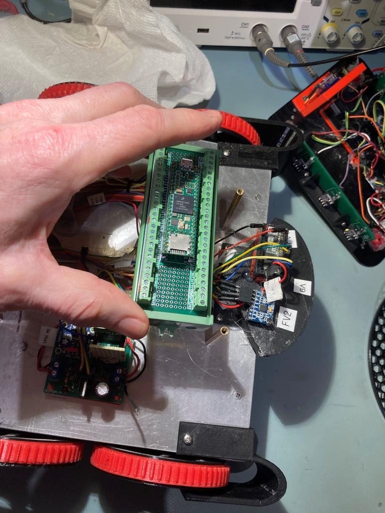
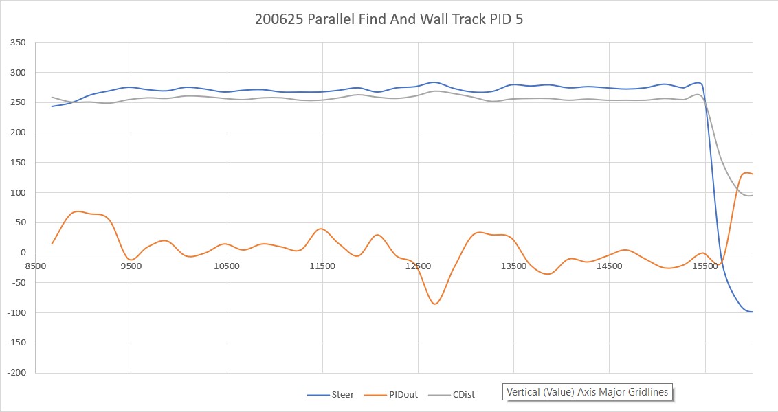
Earlier this month I was able to demonstrate a multi-lap left-side wall tracking run by Wall-E3 in my office ‘sandbox’. This post describes my efforts to extend this capability to right-side wall tracking.

Since I already had the left-side wall tracking algorithm “in the can”, I thought it would be a piece of cake to extend this capability to right-side tracking. Little did I know that this would turn into yet another adventure in Wonderland – but at least when I finally made it back out of the rabbit-hole, the result was a distinct improvement over the left-side algorithm I started with. Here’s the left-side code:

void TrackLeftWallOffset(float kp, float ki, float kd, float offsetCm)
{
  //Purpose: Track left wall at specified offset
  // Inputs:
  //  kp,ki,kd = float objects denoting PID parameters for PIDCalcs()
  //  offsetCm = float denoting desired wall offset, in Cm
  // Plan:
  //  Step1: If robot is already close to desired offset, just turn parallel and go
  //  Step1: Otherwise, get current robot orientation and offset wrt wall
  //  Step2: Move to offset distance and parallel to wall
  //  Step3: Track wall at desired offset 
  //Notes:
  //	06/21/21 modified to do a turn, then straight, then track 0 steer val

  mSecSinceLastWallTrackUpdate = 0;
  float lastError = 0;
  float lastInput = 0;
  float lastIval = 0;
  float lastDerror = 0;
  float spinRateDPS = 30;

  AnomalyCode errcode = NO_ANOMALIES;//03/06/22 mvd here to make global to function

  GetRequestedVL53l0xValues(VL53L0X_LEFT); //update glLeftSteeringVal

  myTeePrint.printf("\nIn TrackLeftWallOffset with Kp/Ki/Kd = %2.2f\t%2.2f\t%2.2f\n", kp, ki, kd);
  myTeePrint.printf("\nIn TrackLeftWallOffset with LR/LC/LF = %d\t%d\t%d\n", glLeftRearCm, glLeftCenterCm, glLeftFrontCm);

//Step1: If robot is already close to desired offset, just turn parallel and go
  if (abs(WALL_OFFSET_TGTDIST_CM - glLeftCenterCm) <= (uint16_t)((float)WALL_OFFSET_TGTDIST_CM/10.f))
  {
    myTeePrint.printf("At %d with desired offset = %d: close enough  - just parallel and go\n", 
      glLeftCenterCm, WALL_OFFSET_TGTDIST_CM);

    RotateToParallelOrientation(TRACKING_LEFT);
  }
  else //OK, have to move to offset distance before rotating back to parallel
  {
    //Step1: Get current robot orientation and offset wrt wall
    float cutAngleDeg = WALL_OFFSET_TGTDIST_CM - (int)(glLeftCenterCm);//positive inside, negative outside desired offset
    //myTeePrint.printf("R/C/F dists = %d\t%d\t%d Steerval = %2.3f, CutAngle = %2.2f\n",
    //  glLeftRearCm, glLeftCenterCm, glLeftFrontCm, glLeftSteeringVal, cutAngleDeg);

    //07/05/21 implement min cut angle
    if (cutAngleDeg < 0 && abs(cutAngleDeg) < WALL_OFFSET_APPR_ANGLE_MINDEG)
    {
      //myTeePrint.printf("(cutAngleDeg < 0 && abs(cutAngleDeg) < %d -- setting to -%d\n", WALL_OFFSET_APPR_ANGLE_MINDEG, WALL_OFFSET_APPR_ANGLE_MINDEG);
      cutAngleDeg = -WALL_OFFSET_APPR_ANGLE_MINDEG;
    }
    else if (cutAngleDeg > 0 && cutAngleDeg < WALL_OFFSET_APPR_ANGLE_MINDEG)
    {
      //myTeePrint.printf("(cutAngleDeg > 0 && abs(cutAngleDeg) < %d -- setting to +%d\n", WALL_OFFSET_APPR_ANGLE_MINDEG, WALL_OFFSET_APPR_ANGLE_MINDEG);
      cutAngleDeg = WALL_OFFSET_APPR_ANGLE_MINDEG;
    }

    //Step2: get the steering angle from the steering value, for comparison to the computed cut angle
    //positive value means robot is oriented away from wall
    float WallOrientDeg = GetWallOrientDeg(glLeftSteeringVal);

    //myTeePrint.printf("R/C/F dists = %d\t%d\t%d Steerval = %2.3f, SteerAngle = %2.2f, CutAngle = %2.2f\n",
    //  glLeftRearCm, glLeftCenterCm, glLeftFrontCm, glLeftSteeringVal, WallOrientDeg, cutAngleDeg);

    //Step3: now decide which way to turn.
    int16_t fudgeFactorCm = 0; //07/05/21 added so can change for inside vs outside starting condx
    if (cutAngleDeg > 0) //robot inside desired offset distance
    {
      if (WallOrientDeg > cutAngleDeg)  // --> WallOrientDeg also > 0, have to turn CCW
      {
        //myTeePrint.printf("CutAngDeg > 0, WallOrientDeg > cutAngleDeg - Turn CCW to cut angle\n");
        SpinTurn(true, WallOrientDeg - cutAngleDeg, spinRateDPS); //
      }
      else //(WallOrientDeg <= cutAngleDeg)// --> WallOrientDeg could be < 0
      {
        //myTeePrint.printf("CutAngDeg > 0, WallOrientDeg < cutAngleDeg\n");
        SpinTurn(false, cutAngleDeg - WallOrientDeg, spinRateDPS); //turn diff between WallOrientDeg & cutAngleDeg
      }

      fudgeFactorCm = -10; //07/05/21 don't need fudge factor for inside start condx
    }
    else // cutAngleDeg < 0 --> robot outside desired offset distance
    {
      if (WallOrientDeg > cutAngleDeg)  // --> WallOrientDeg may also be > 0
      {
        //robot turned too far toward wall
        myTeePrint.printf("CutAngDeg < 0, WallOrientDeg > cutAngleDeg\n");
        SpinTurn(true, WallOrientDeg - cutAngleDeg, spinRateDPS); //
      }
      else// (WallOrientDeg < cutAngleDeg)// --> WallOrientDeg must also be < 0
      {
        //robot turned to far away from wall
        myTeePrint.printf("CutAngDeg < 0, WallOrientDeg <= 0\n");
        SpinTurn(false, cutAngleDeg - WallOrientDeg, spinRateDPS); //null out WallOrientDeg & then turn addnl cutAngleDeg
      }

      fudgeFactorCm = 10; //07/05/21 need fudge factor for outside start condx
    }

    //myTeePrint.printf("fudgeFactorCm = %d\n", fudgeFactorCm);
    //delay(1000);

    //Step4: Figure out how far to travel to get to desired offset
    //adjust so offset capture occurs at correct perpendicular offset
    float adjfactor = cos(PI * cutAngleDeg / 180.f);
    float numerator = (float)WALL_OFFSET_TGTDIST_CM;
    float adjOffsetCm = (numerator / adjfactor);
    adjOffsetCm += fudgeFactorCm; //fudge factor for distance measurements lagging behind robot's travel. 
    //myTeePrint.printf("\nat approach start: cut angle = %2.3f, adjfactor = %2.3f, num = %2.2f, adjOffsetCm = %2.2f\n",
      //cutAngleDeg, adjfactor, numerator, adjOffsetCm);

    GetRequestedVL53l0xValues(VL53L0X_ALL); //added 09/05/21
    int16_t err = glLeftFrontCm - (uint16_t)adjOffsetCm; //neg for inside going out, pos for outside going in
    int16_t prev_err = err;
    //myTeePrint.printf("At start - err = prev_err = %ld\n", err, prev_err);

    WallOrientDeg = GetWallOrientDeg(glLeftSteeringVal);
    myTeePrint.printf("R/C/F dists = %d\t%d\t%d Steerval = %2.3f, SteerAngle = %2.2f, CutAngle = %2.2f, err/prev_err = %li\n",
      glLeftRearCm, glLeftCenterCm, glLeftFrontCm, glLeftSteeringVal, WallOrientDeg, cutAngleDeg, err);


    //myTeePrint.printf("Msec\tLFront\tLCtr\tLRear\tFront\tRear\tErr\tP_err\n");

    //Step5: Move to desired offset
    //02/25/22 added check for error conditions (stuck, obstacle, dead battery, etc)
    AnomalyCode errcode = NO_ANOMALIES;
    while (((cutAngleDeg > 0 && err < 0) || (cutAngleDeg <= 0 && err >= 0)) && prev_err * err > 0 && errcode == NO_ANOMALIES) //sign change makes this < 0
    {
      prev_err = err;

      //MoveAhead(MOTOR_SPEED_FULL, MOTOR_SPEED_FULL);
      MoveAhead(MOTOR_SPEED_HALF, MOTOR_SPEED_HALF);
      delay(100);
      glFrontdistval = GetFrontDistCm();
      GetRequestedVL53l0xValues(VL53L0X_ALL);
      err = glLeftFrontCm - adjOffsetCm; //06/29/21 now adj for slant dist vs perp dist
      //myTeePrint.printf("%lu\t%d\t%d\t%d\t%d\t%d\t%ld\t%ld\n",
      //  millis(),
      //  glLeftFrontCm, glLeftCenterCm, glLeftRearCm, glFrontdistval, glRearCm, err, prev_err);

      CheckForUserInput();
      errcode = CheckForErrorCondx();
    }

    //Step6: now turn back the same (unadjusted) amount
    //myTeePrint.printf("At end of offset capture - prev_res*res = %ld\n", prev_err * err);
    //myTeePrint.printf("correct back to parallel (left side)\n");
    SpinTurn(!(cutAngleDeg < 0), abs(cutAngleDeg), spinRateDPS); //have to use abs() here, as cutAngleDeg can be neg
  }
  WallTrackSetPoint = 0; //moved here 6/22/21

  myTeePrint.printf("\nTrackLeftWallOffset: Start tracking offset of %2.2fcm with Kp/Ki/Kd = %2.2f\t%2.2f\t%2.2f\n", offsetCm, kp, ki, kd);
  //myTeePrint.printf("Msec\tFdir\tCdir\tRdir\tRearD\tSteer\tSet\terror\tIval\tKp*err\tKi*Ival\tKd*Din\tOutput\tLspd\tRspd\n");
  myTeePrint.printf("Msec\tLF\tLC\tLR\t\tRF\tRC\tRR\t\tF\tFvar\t\tR\tRvar\t\tSteer\tSet\tOutput\n");

  //Step7: Track the wall using PID algorithm
  mSecSinceLastWallTrackUpdate = 0; //added 09/04/21
  while (errcode == NO_ANOMALIES)
  {
    CheckForUserInput(); //this is a bit recursive, but should still work (I hope)

    //09/04/21 back to elapsedMillis timing
    if (mSecSinceLastWallTrackUpdate > WALL_TRACK_UPDATE_INTERVAL_MSEC)
    {
      digitalToggle(DURATION_MEASUREMENT_PIN2); //03/08/22 toggle duration measurement pulse

      mSecSinceLastWallTrackUpdate -= WALL_TRACK_UPDATE_INTERVAL_MSEC;

      //03/08/22 abstracted these calls to UpdateAllEnvironmentParameters()
      UpdateAllEnvironmentParameters();//03/08/22 added to consolidate sensor update calls
      errcode = CheckForErrorCondx();

      //have to weight value by both angle and wall offset
      WallTrackSteerVal = glLeftSteeringVal + (glLeftCenterCm - WALL_OFFSET_TGTDIST_CM) / 1000.f;

      //update motor speeds, skipping bad values
      if (!isnan(WallTrackSteerVal))
      {
        WallTrackOutput = PIDCalcs(WallTrackSteerVal, WallTrackSetPoint, lastError, lastInput, lastIval, lastDerror,
          kp, ki, kd);

        int glLeftspeednum = MOTOR_SPEED_QTR + WallTrackOutput;
        int glRightspeednum = MOTOR_SPEED_QTR - WallTrackOutput;

        glRightspeednum = (glRightspeednum <= MOTOR_SPEED_HALF) ? glRightspeednum : MOTOR_SPEED_HALF;
        glRightspeednum = (glRightspeednum > 0) ? glRightspeednum : 0;
        glLeftspeednum = (glLeftspeednum <= MOTOR_SPEED_HALF) ? glLeftspeednum : MOTOR_SPEED_HALF;
        glLeftspeednum = (glLeftspeednum > 0) ? glLeftspeednum : 0;

        MoveAhead(glLeftspeednum, glRightspeednum);

        //myTeePrint.printf("Msec\tLF\tLC\tLR\t\tRF\tRC\tRR\t\tF\tFvar\tR\tRvar\t\tSteer\tSet\tOutput\n");
        myTeePrint.printf("%lu\t%d\t%d\t%d\t\t%d\t%d\t%d\t\t%d\t%d\t%2.2f\t%2.2f\t\t%2.2f\t%2.2f\t%2.2f\n",
          millis(),
          glLeftFrontCm, glLeftCenterCm, glLeftRearCm,
          glRightFrontCm, glRightCenterCm, glRightRearCm, 
          glFrontdistval, glFrontvar, glRearCm, glRearvar,
          WallTrackSteerVal, WallTrackSetPoint, WallTrackOutput);
      }
      digitalToggle(DURATION_MEASUREMENT_PIN2); //03/08/22 toggle duration measurement pulse

    }
  }

  //Step8: Handle any anomalous conditions
  HandleAnomalousConditions(errcode, TRACKING_LEFT);
}

100

101

102

103

104

105

106

107

108

109

110

111

112

113

114

115

116

117

118

119

120

121

122

123

124

125

126

127

128

129

130

131

132

133

134

135

136

137

138

139

140

141

142

143

144

145

146

147

148

149

150

151

152

153

154

155

156

157

158

159

160

161

162

163

164

165

166

167

168

169

170

171

172

173

174

175

176

177

178

179

180

181

182

183

184

185

186

187

188

189

190

191

192

193

194

195

196

197

198

199

200

201

202

203

204

205

void TrackLeftWallOffset(float kp, float ki, float kd, float offsetCm)

{

//Purpose: Track left wall at specified offset

// Inputs:

// kp,ki,kd = float objects denoting PID parameters for PIDCalcs()

// offsetCm = float denoting desired wall offset, in Cm

// Plan:

// Step1: If robot is already close to desired offset, just turn parallel and go

// Step1: Otherwise, get current robot orientation and offset wrt wall

// Step2: Move to offset distance and parallel to wall

// Step3: Track wall at desired offset

//Notes:

// 06/21/21 modified to do a turn, then straight, then track 0 steer val

mSecSinceLastWallTrackUpdate = 0;

float lastError = 0;

float lastInput = 0;

float lastIval = 0;

float lastDerror = 0;

float spinRateDPS = 30;

AnomalyCode errcode = NO_ANOMALIES;//03/06/22 mvd here to make global to function

GetRequestedVL53l0xValues(VL53L0X_LEFT); //update glLeftSteeringVal

myTeePrint.printf("\nIn TrackLeftWallOffset with Kp/Ki/Kd = %2.2f\t%2.2f\t%2.2f\n", kp, ki, kd);

myTeePrint.printf("\nIn TrackLeftWallOffset with LR/LC/LF = %d\t%d\t%d\n", glLeftRearCm, glLeftCenterCm, glLeftFrontCm);

//Step1: If robot is already close to desired offset, just turn parallel and go

if (abs(WALL_OFFSET_TGTDIST_CM - glLeftCenterCm) <= (uint16_t)((float)WALL_OFFSET_TGTDIST_CM/10.f))

{

myTeePrint.printf("At %d with desired offset = %d: close enough - just parallel and go\n",

glLeftCenterCm, WALL_OFFSET_TGTDIST_CM);

RotateToParallelOrientation(TRACKING_LEFT);

}

else //OK, have to move to offset distance before rotating back to parallel

{

//Step1: Get current robot orientation and offset wrt wall

float cutAngleDeg = WALL_OFFSET_TGTDIST_CM - (int)(glLeftCenterCm);//positive inside, negative outside desired offset

//myTeePrint.printf("R/C/F dists = %d\t%d\t%d Steerval = %2.3f, CutAngle = %2.2f\n",

// glLeftRearCm, glLeftCenterCm, glLeftFrontCm, glLeftSteeringVal, cutAngleDeg);

//07/05/21 implement min cut angle

if (cutAngleDeg < 0 && abs(cutAngleDeg) < WALL_OFFSET_APPR_ANGLE_MINDEG)

{

//myTeePrint.printf("(cutAngleDeg < 0 && abs(cutAngleDeg) < %d -- setting to -%d\n", WALL_OFFSET_APPR_ANGLE_MINDEG, WALL_OFFSET_APPR_ANGLE_MINDEG);

cutAngleDeg = -WALL_OFFSET_APPR_ANGLE_MINDEG;

}

else if (cutAngleDeg > 0 && cutAngleDeg < WALL_OFFSET_APPR_ANGLE_MINDEG)

{

//myTeePrint.printf("(cutAngleDeg > 0 && abs(cutAngleDeg) < %d -- setting to +%d\n", WALL_OFFSET_APPR_ANGLE_MINDEG, WALL_OFFSET_APPR_ANGLE_MINDEG);

cutAngleDeg = WALL_OFFSET_APPR_ANGLE_MINDEG;

}

//Step2: get the steering angle from the steering value, for comparison to the computed cut angle

//positive value means robot is oriented away from wall

float WallOrientDeg = GetWallOrientDeg(glLeftSteeringVal);

//myTeePrint.printf("R/C/F dists = %d\t%d\t%d Steerval = %2.3f, SteerAngle = %2.2f, CutAngle = %2.2f\n",

// glLeftRearCm, glLeftCenterCm, glLeftFrontCm, glLeftSteeringVal, WallOrientDeg, cutAngleDeg);

//Step3: now decide which way to turn.

int16_t fudgeFactorCm = 0; //07/05/21 added so can change for inside vs outside starting condx

if (cutAngleDeg > 0) //robot inside desired offset distance

{

if (WallOrientDeg > cutAngleDeg) // --> WallOrientDeg also > 0, have to turn CCW

{

//myTeePrint.printf("CutAngDeg > 0, WallOrientDeg > cutAngleDeg - Turn CCW to cut angle\n");

SpinTurn(true, WallOrientDeg - cutAngleDeg, spinRateDPS); //

}

else //(WallOrientDeg <= cutAngleDeg)// --> WallOrientDeg could be < 0

{

//myTeePrint.printf("CutAngDeg > 0, WallOrientDeg < cutAngleDeg\n");

SpinTurn(false, cutAngleDeg - WallOrientDeg, spinRateDPS); //turn diff between WallOrientDeg & cutAngleDeg

}

fudgeFactorCm = -10; //07/05/21 don't need fudge factor for inside start condx

}

else // cutAngleDeg < 0 --> robot outside desired offset distance

{

if (WallOrientDeg > cutAngleDeg) // --> WallOrientDeg may also be > 0

{

//robot turned too far toward wall

myTeePrint.printf("CutAngDeg < 0, WallOrientDeg > cutAngleDeg\n");

SpinTurn(true, WallOrientDeg - cutAngleDeg, spinRateDPS); //

}

else// (WallOrientDeg < cutAngleDeg)// --> WallOrientDeg must also be < 0

{

//robot turned to far away from wall

myTeePrint.printf("CutAngDeg < 0, WallOrientDeg <= 0\n");

SpinTurn(false, cutAngleDeg - WallOrientDeg, spinRateDPS); //null out WallOrientDeg & then turn addnl cutAngleDeg

}

fudgeFactorCm = 10; //07/05/21 need fudge factor for outside start condx

}

//myTeePrint.printf("fudgeFactorCm = %d\n", fudgeFactorCm);

//delay(1000);

//Step4: Figure out how far to travel to get to desired offset

//adjust so offset capture occurs at correct perpendicular offset

float adjfactor = cos(PI * cutAngleDeg / 180.f);

float numerator = (float)WALL_OFFSET_TGTDIST_CM;

float adjOffsetCm = (numerator / adjfactor);

adjOffsetCm += fudgeFactorCm; //fudge factor for distance measurements lagging behind robot's travel.

//myTeePrint.printf("\nat approach start: cut angle = %2.3f, adjfactor = %2.3f, num = %2.2f, adjOffsetCm = %2.2f\n",

//cutAngleDeg, adjfactor, numerator, adjOffsetCm);

GetRequestedVL53l0xValues(VL53L0X_ALL); //added 09/05/21

int16_t err = glLeftFrontCm - (uint16_t)adjOffsetCm; //neg for inside going out, pos for outside going in

int16_t prev_err = err;

//myTeePrint.printf("At start - err = prev_err = %ld\n", err, prev_err);

WallOrientDeg = GetWallOrientDeg(glLeftSteeringVal);

myTeePrint.printf("R/C/F dists = %d\t%d\t%d Steerval = %2.3f, SteerAngle = %2.2f, CutAngle = %2.2f, err/prev_err = %li\n",

glLeftRearCm, glLeftCenterCm, glLeftFrontCm, glLeftSteeringVal, WallOrientDeg, cutAngleDeg, err);

//myTeePrint.printf("Msec\tLFront\tLCtr\tLRear\tFront\tRear\tErr\tP_err\n");

//Step5: Move to desired offset

//02/25/22 added check for error conditions (stuck, obstacle, dead battery, etc)

AnomalyCode errcode = NO_ANOMALIES;

while (((cutAngleDeg > 0 && err < 0) || (cutAngleDeg <= 0 && err >= 0)) && prev_err * err > 0 && errcode == NO_ANOMALIES) //sign change makes this < 0

{

prev_err = err;

//MoveAhead(MOTOR_SPEED_FULL, MOTOR_SPEED_FULL);

MoveAhead(MOTOR_SPEED_HALF, MOTOR_SPEED_HALF);

delay(100);

glFrontdistval = GetFrontDistCm();

GetRequestedVL53l0xValues(VL53L0X_ALL);

err = glLeftFrontCm - adjOffsetCm; //06/29/21 now adj for slant dist vs perp dist

//myTeePrint.printf("%lu\t%d\t%d\t%d\t%d\t%d\t%ld\t%ld\n",

// millis(),

// glLeftFrontCm, glLeftCenterCm, glLeftRearCm, glFrontdistval, glRearCm, err, prev_err);

CheckForUserInput();

errcode = CheckForErrorCondx();

}

//Step6: now turn back the same (unadjusted) amount

//myTeePrint.printf("At end of offset capture - prev_res*res = %ld\n", prev_err * err);

//myTeePrint.printf("correct back to parallel (left side)\n");

SpinTurn(!(cutAngleDeg < 0), abs(cutAngleDeg), spinRateDPS); //have to use abs() here, as cutAngleDeg can be neg

}

WallTrackSetPoint = 0; //moved here 6/22/21

myTeePrint.printf("\nTrackLeftWallOffset: Start tracking offset of %2.2fcm with Kp/Ki/Kd = %2.2f\t%2.2f\t%2.2f\n", offsetCm, kp, ki, kd);

//myTeePrint.printf("Msec\tFdir\tCdir\tRdir\tRearD\tSteer\tSet\terror\tIval\tKp*err\tKi*Ival\tKd*Din\tOutput\tLspd\tRspd\n");

myTeePrint.printf("Msec\tLF\tLC\tLR\t\tRF\tRC\tRR\t\tF\tFvar\t\tR\tRvar\t\tSteer\tSet\tOutput\n");

//Step7: Track the wall using PID algorithm

mSecSinceLastWallTrackUpdate = 0; //added 09/04/21

while (errcode == NO_ANOMALIES)

{

CheckForUserInput(); //this is a bit recursive, but should still work (I hope)

//09/04/21 back to elapsedMillis timing

if (mSecSinceLastWallTrackUpdate > WALL_TRACK_UPDATE_INTERVAL_MSEC)

{

digitalToggle(DURATION_MEASUREMENT_PIN2); //03/08/22 toggle duration measurement pulse

mSecSinceLastWallTrackUpdate -= WALL_TRACK_UPDATE_INTERVAL_MSEC;

//03/08/22 abstracted these calls to UpdateAllEnvironmentParameters()

UpdateAllEnvironmentParameters();//03/08/22 added to consolidate sensor update calls

errcode = CheckForErrorCondx();

//have to weight value by both angle and wall offset

WallTrackSteerVal = glLeftSteeringVal + (glLeftCenterCm - WALL_OFFSET_TGTDIST_CM) / 1000.f;

//update motor speeds, skipping bad values

if (!isnan(WallTrackSteerVal))

{

WallTrackOutput = PIDCalcs(WallTrackSteerVal, WallTrackSetPoint, lastError, lastInput, lastIval, lastDerror,

kp, ki, kd);

int glLeftspeednum = MOTOR_SPEED_QTR + WallTrackOutput;

int glRightspeednum = MOTOR_SPEED_QTR - WallTrackOutput;

glRightspeednum = (glRightspeednum <= MOTOR_SPEED_HALF) ? glRightspeednum : MOTOR_SPEED_HALF;

glRightspeednum = (glRightspeednum > 0) ? glRightspeednum : 0;

glLeftspeednum = (glLeftspeednum <= MOTOR_SPEED_HALF) ? glLeftspeednum : MOTOR_SPEED_HALF;

glLeftspeednum = (glLeftspeednum > 0) ? glLeftspeednum : 0;

MoveAhead(glLeftspeednum, glRightspeednum);

//myTeePrint.printf("Msec\tLF\tLC\tLR\t\tRF\tRC\tRR\t\tF\tFvar\tR\tRvar\t\tSteer\tSet\tOutput\n");

myTeePrint.printf("%lu\t%d\t%d\t%d\t\t%d\t%d\t%d\t\t%d\t%d\t%2.2f\t%2.2f\t\t%2.2f\t%2.2f\t%2.2f\n",

millis(),

glLeftFrontCm, glLeftCenterCm, glLeftRearCm,

glRightFrontCm, glRightCenterCm, glRightRearCm,

glFrontdistval, glFrontvar, glRearCm, glRearvar,

WallTrackSteerVal, WallTrackSetPoint, WallTrackOutput);

}

digitalToggle(DURATION_MEASUREMENT_PIN2); //03/08/22 toggle duration measurement pulse

}

//Step8: Handle any anomalous conditions

HandleAnomalousConditions(errcode, TRACKING_LEFT);

}

The above code works, in the sense that it allows Wall-E3 to successfully track the left-side wall of my ‘sandbox’. However, as I worked on porting the left-side tracking code to the right side, I kept thinking – this is awful code – surely there is a better way?

After letting this problem percolate for few days, I decided to see if I could approach the problem a little more logically. I realized there were two major conditions associated with the problem – namely is the robot’s initial position inside or outside the desired offset distance K? In addition, the robot can start out parallel to the wall, or pointed toward or away from the wall. Ignoring the ‘started out parallel’ degenerate case, this reminded me of a 3-parameter Karnaugh map configuration, so I started sketching it out in my notebook, and then later in a Word document, as shown below:

As shown above, I broke the 3-parameter into two 2-parameter Karnaugh maps, and the output is denoted by α_T. After a few minutes it became obvious that the formula for α_T is pretty simple – its either α_R – α_A1 or α_R – α_A2depending on whether the robot starts out outside or inside the desired offset distance. In code, this boils down to one line, as shown at the bottom of the Karnaugh map above, using the C++ ‘?’ trinary operator, and choosing CW vs CCW is easy too, as a negative result implies CCW, and a positive one implies CW. The actual code block is shown below:

    //Step3: now decide which way to turn.
    float turndeg = 0; 
    float appAngle = 0;
    if (bInsideOffset) //approach angle = +30
    {
      appAngle = 30;
      turndeg = WallOrientDeg - appAngle;
      fudgeFactorCm = -10;
    }
    else
    {
      appAngle = -30;
      turndeg = WallOrientDeg - appAngle;
      fudgeFactorCm = 10; 
    }

    SpinTurn((turndeg < 0), abs(turndeg));

//Step3: now decide which way to turn.

float turndeg = 0;

float appAngle = 0;

if (bInsideOffset) //approach angle = +30

{

appAngle = 30;

turndeg = WallOrientDeg - appAngle;

fudgeFactorCm = -10;

}

else

{

appAngle = -30;

turndeg = WallOrientDeg - appAngle;

fudgeFactorCm = 10;

}

SpinTurn((turndeg < 0), abs(turndeg));

Here’s a short video of Wall-E3 navigating the office ‘sandbox’ while tracking the right-side wall.

So, it looks like Wall-E3 now has tracking ability for both left-side and right-side walls, although I still have to clean things up and port the simpler right-side code into TrackLeftWallOffset().

25 March 2022 Update:

Well, that was easy! I just got through porting the new right-side wall tracking algorithm over to TrackLeftWallOffset(), and right out of the box was able to demonstrate successful left-wall tracking in my office ‘sandbox’.

At this point I believe I’m going to consider the ‘WallE3_WallTrack_V3’ project ‘finished’ (in the sense that most, if not all, my wall tracking goals have been met with this version), and move on to V4, thereby limiting the possible damage from my next inevitable descent through the rabbit hole into wonderland.

Stay tuned,

Frank

Teensy 4.1 Replacement for Teensy 3.5?

Leave a reply

A while back, I had some problems with damaged Teensy 3.5 main controllers on Wall-E3, my autonomous wall-following robot. I eventually traced the problem back to large voltage transients that occurred when I connected/disconnected the charging probe. These transients were conducted to the Teensy 3.5 pin used to detect the probe connection status, causing the Teensy to immediately reboot, and then eventually become unusable. I solved this problem by using a non-conductive photonic charger connect/disconnect system using the supplied charge LED on the TP5100 charger coupled to a photoresistor.

Unfortunately, I ran through most of my Teensy 3.5 stock while I was figuring this out, and now this part is unavailable from PJRC or anywhere else – maybe a victim of the world-wide chip shortage? The good news though is that the Teensys 4.1, successor to the Teensy 3.5 is available, so I purchased a few to evaluate as a replacement for the T3.5 on my robot.

The Teensy 4.1 has the same form factor and pin layout as the T3.5, which means it is a drop-in replacement in most cases. However, there are some gotchas. According to the comparison sheet on Paul Stoffregen’s PJRC site, the T4.1 is 5X faster (600MHz vs 120MHz) and has more memory. However, it doesn’t have any analog output DACs (T3.5 has 2), and more importantly, the T4.1 pins are not 5V tolerant!

To start my evaluation, I loaded a simple ‘blink’ program, and as expected it worked great. Here’s the test setup, utilizing my newly-discovered OONO breakout board.

After this first test, I am convinced that the T4.1 will work nicely as a T3.5 replacement, except possibly for the 5V tolerance issue. To investigate this, I looked at my current system schematic

Wall-E3’s main controller is directly connected to two VNH5019 motor controllers, several LEDs (the Chg Stat Display module), two INA169 current sense modules, a Pulsed Light (now owned by Garmin) LIDAR system via it’s ‘Mode’ pin, the ‘HC-05 BT Module’ (now replaced by my new 5V Reg/Wixel board) via its TX/RX pins, and the battery pack via the ‘Chg Conn’ pin (this the photonic connection discussed above). It is also connected to a MPU6050 IMU, a Teensy 3.2 running the IR charging beam detector, and another Teensy 3.5 running the 7-element VL53L0X distance sensing array, all via two different I2C ports.

The I2C ports are no problem, as they are either Teensy-to-Teensy or Teensy-to-MPU6050, which has an onboard regulator to regulate 5V down to 3.3, so the data lanes are 3.3V. The LED panels is passive (doesn’t generate any signals of its own), so that’s not a problem. The Wixel RF Transceiver inside my 5V Regulator/Wixel module runs on 3.3V, so the RX/TX lines are compatible with Teensy 4.1. The ‘Irun’, ‘Itot’ and ‘BattV’ A/D inputs are all below 3.3V at their maximum values (The Irun and Itot lines max out at about 2V (2 amps through the current sensor), while BattV maxes out at about 2.4V (8.4V max battery voltage minus 6V drop through a 6V zener diode).

The ‘Mode’ line on the LIDAR could be an issue. The original Pulsed Light LIDAR was acquired by Garmin, so the original datasheets are no longer available. The Garmin datasheet says that the MODE pin output is limited to 3.3V, but I don’t know if that is the same for the original Pulsed Light model I’m using on Wall-E3. So, I hooked up my digital O’scope to the LIDAR’s MODE pin on Wall-E3 and measured it directly. As shown in the following scope grab, the output is indeed limited to 3.3V – yay!

Pulsed Light LIDAR-Lite MODE pin pulse output. Note max amplitude (Ma) = 3.308V

So, it looks like I can drop a Teensy 4.1 into Wall-E3’s system and it should do fine. I don’t really need the speed and/or memory improvements, but I do need a replacement for the now-defunct Teensy 3.5, in case I manage to kill yet another one.

21 March 2022 Update:

I took the time today to see how (or if) the Teensy 4.1 breakout module would fit on my current Wall-E3 robot. As shown below, it’s pretty big!

Based on the above photos, I don’t think this breakout board has a future on Wall-E3. Even though the module will fit, that doesn’t take into account the fact that the wiring from the module will extend horizontally from the module, rather than vertically as it does with the plain ‘Teensy + Female header’ arrangement. It was a great idea a the time, but I guess the reality is that the breakout module will be relegated to testing,

Stay tuned,

Frank

Wall-E3 Replacing Mega 2560 With Teensy 3.5 Part VIII

Leave a reply

Posted 19 February 2022,

At this point in the evolution of Wall-E3, all the hardware seems to be working, so it’s time to get serious about wall tracking. Last fall I made another run at wall tracking with Wall-E2, and wound up with an algorithm that would first capture the desired wall offset, and then track it ‘forever’. This worked great, but the approach is at odds with the general processing architecture. The current tracking architecture is set up as a loop, where all pertinent parameters are updated every loop period, and the appropriate action is taken. In the case of wall tracking, the ‘action’ was one left/right motor speed update. This allows rapid recognition of, and adaptation to, various ‘error’ conditions, like being stuck or about to run into something. The algorithm developed last fall does none of this, so it can’t react properly (or at all, for that matter) to things like an upcoming wall.

I’m starting to think I can use a hybrid approach – use the current capture/tracking algorithm pretty much as it stands from last fall, but have it check for ‘error’ conditions each time through its own internal loop. If any unusual conditions are detected, then force an exit from the tracking routine and another pass through the main ‘traffic director’ function ‘GetOpMode()’. The updated mode assignment will then percolate back down through loop() and cause the appropriate handling function to be called.

22 February 2022 Update:

As a start, I ported the ‘TrackLeft/RightWallOffset() functions to Wall-E3 and, after the normal number of screwups and mistakes, I got the left side tracking algorithm working, as shown in the Excel plot and short movie clip below:

Here’s the complete code for ‘TrackLeftWallOffset()’:

void TrackRightWallOffset(float kp, float ki, float kd, float offsetCm)
{
  //Notes:
  //	06/21/21 modified to do a turn, then straight, then track 0 steer val
  //	09/12/21 updated from TrackLeftWallOffset
  //  02/22/22 cleaned up

  mSecSinceLastWallTrackUpdate = 0;
  float lastError = 0;
  float lastInput = 0;
  float lastIval = 0;
  float lastDerror = 0;
  float spinRateDPS = 30;

  GetRequestedVL53l0xValues(VL53L0X_RIGHT); //update glRightSteeringVal = (Front - Rear)/100

  //09/12/21 ported from TrackLeftWallOffset
  myTeePrint.printf("\nIn TrackRightWallOffset with Kp/Ki/Kd = %2.2f\t%2.2f\t%2.2f\n", kp, ki, kd);

  //06/21/21 modified to do a turn, then straight, then track 0 steer val
  float cutAngleDeg = WALL_OFFSET_TGTDIST_CM - (int)(glLidar_RightCenter / 10.f);//positive inside, negative outside desired offset
  myTeePrint.printf("R/C/F dists = %d\t%d\t%d Steerval = %2.3f, CutAngle = %2.2f\n",
    glLidar_RightRear, glLidar_RightCenter, glLidar_RightFront, glRightSteeringVal, cutAngleDeg);

  //07/05/21 implement min cut angle
  if (cutAngleDeg < 0 && abs(cutAngleDeg) < WALL_OFFSET_APPR_ANGLE_MINDEG)
  {
    myTeePrint.printf("(cutAngleDeg < 0 && abs(cutAngleDeg) < %d -- setting to -%d\n", WALL_OFFSET_APPR_ANGLE_MINDEG, WALL_OFFSET_APPR_ANGLE_MINDEG);
    cutAngleDeg = -WALL_OFFSET_APPR_ANGLE_MINDEG;
  }
  else if (cutAngleDeg > 0 && cutAngleDeg < WALL_OFFSET_APPR_ANGLE_MINDEG)
  {
    myTeePrint.printf("(cutAngleDeg > 0 && abs(cutAngleDeg) < %d -- setting to +%d\n", WALL_OFFSET_APPR_ANGLE_MINDEG, WALL_OFFSET_APPR_ANGLE_MINDEG);
    cutAngleDeg = WALL_OFFSET_APPR_ANGLE_MINDEG;
  }

  //get the steering angle from the steering value, for comparison to the computed cut angle
  //positive value means robot is oriented away from wall
  float SteerAngleDeg = GetSteeringAngle(glRightSteeringVal);

  myTeePrint.printf("R/C/F dists = %d\t%d\t%d Steerval = %2.3f, SteerAngle = %2.2f, CutAngle = %2.2f\n",
    glLidar_RightRear, glLidar_RightCenter, glLidar_RightFront, glRightSteeringVal, SteerAngleDeg, cutAngleDeg);

  //now decide which way to turn.
  //double adjCutAngleDeg = 0;
  uint16_t fudgeFactorMM = 0; //07/05/21 added so can change for inside vs outside starting condx
  if (cutAngleDeg > 0) //robot inside desired offset distance
  {
    if (SteerAngleDeg > cutAngleDeg)  // --> implies SteerAngleDeg also > 0
    {
      //robot pointed away from wall more than it should
      myTeePrint.printf("CutAngDeg > 0, SteerAngleDeg > cutAngleDeg\n");
      SpinTurn(false, SteerAngleDeg - cutAngleDeg, spinRateDPS); //turn back toward wall to achieve cutAngle
    }
    else if (SteerAngleDeg < cutAngleDeg)// --> SteerAngleDeg could be < 0
    {
      //robot not turned far enough away from wall (could actually be turned toward wall if SteerAngDeg < 0)
      myTeePrint.printf("CutAngDeg > 0, SteerAngleDeg < cutAngleDeg\n");
      if (SteerAngleDeg <= 0) //cutAngleDeg > 0, SteerAngleDeg <= 0
      {
        //robot turned toward wall
        myTeePrint.printf("CutAngDeg > 0, SteerAngleDeg < cutAngleDeg, SteerAngleDeg <= 0\n");
        SpinTurn(true, cutAngleDeg + SteerAngleDeg, spinRateDPS); //null out SteerAngleDeg & then turn addnl cutAngleDeg
      }
      else //SteerAngleDeg < cutAngleDeg but still > 0
      {
        //robot turned away from wall, but not far enough
        myTeePrint.printf("CutAngDeg > 0,  0 < SteerAngleDeg < cutAngleDeg\n");
        SpinTurn(true, cutAngleDeg - SteerAngleDeg, spinRateDPS); //turn diff between SteerAngleDeg & cutAngleDeg
      }
    }

    fudgeFactorMM = -100; //07/05/21 don't need fudge factor for inside start condx
  }
  else // cutAngleDeg < 0 --> robot outside desired offset distance
  {
    if (SteerAngleDeg < cutAngleDeg)  // --> SteerAngleDeg must also be < 0
    {
      //robot turned too far toward wall
      myTeePrint.printf("CutAngDeg < 0, SteerAngleDeg < cutAngleDeg\n");
      SpinTurn(true, SteerAngleDeg - cutAngleDeg, spinRateDPS); //turn away from wall to achieve cutAngleDeg
    }
    else if (SteerAngleDeg >= cutAngleDeg)// --> SteerAngleDeg could be >=0
    {
      if (SteerAngleDeg >= 0) //cutAngleDeg < 0, SteerAngleDeg >= 0
      {
        //robot turned to far away from wall
        myTeePrint.printf("CutAngDeg < 0, SteerAngleDeg <= 0\n");
        SpinTurn(false, cutAngleDeg + SteerAngleDeg, spinRateDPS); //null out SteerAngleDeg & then turn addnl cutAngleDeg
      }
      else //SteerAngleDeg > cutAngleDeg but still < 0
      {
        //robot turned toward wall, but not enough
        myTeePrint.printf("CutAngDeg < 0, 0 < SteerAngleDeg < cutAngleDeg\n");
        SpinTurn(false, cutAngleDeg - SteerAngleDeg, spinRateDPS); //turn diff between SteerAngleDeg & cutAngleDeg
      }
    }

    fudgeFactorMM = 100; //07/05/21 need fudge factor for outside start condx
  }

  delay(1000);

  //adjust so offset capture occurs at correct perpendicular offset
  float adjfactor = cos(PI * cutAngleDeg / 180.f);
  int adjOffsetMM = (int)(10 * (float)WALL_OFFSET_TGTDIST_CM / adjfactor);
  adjOffsetMM += fudgeFactorMM; //fudge factor for distance measurements lagging behind robot's travel. 
  myTeePrint.printf("\nat approach start: cut angle = %2.3f, adjfactor = %2.3f, tgt dist = %d\n", cutAngleDeg, adjfactor, adjOffsetMM);

  GetRequestedVL53l0xValues(VL53L0X_ALL); //added 09/05/21

  long int err = glLidar_RightFront - adjOffsetMM; //neg for inside going out, pos for outside going in
  long int prev_err = err;
  myTeePrint.printf("At start - err = prev_err = %ld\n", err, prev_err);

  SteerAngleDeg = GetSteeringAngle(glRightSteeringVal);
  myTeePrint.printf("R/C/F dists = %d\t%d\t%d Steerval = %2.3f, SteerAngle = %2.2f, CutAngle = %2.2f, err/prev_err = %li\n",
    glLidar_RightRear, glLidar_RightCenter, glLidar_RightFront, glRightSteeringVal, SteerAngleDeg, cutAngleDeg, err);

  myTeePrint.printf("Msec\tRFront\tRCtr\tRRear\tFront\tRear\tErr\tP_err\n");

  //09/05/21 rev to doublecheck robot position - might not need the forward motion section
  while (((cutAngleDeg > 0 && err < 0) || (cutAngleDeg <= 0 && err >= 0)) && prev_err * err > 0) //sign change makes this < 0
  {
    prev_err = err;

    MoveAhead(MOTOR_SPEED_QTR, MOTOR_SPEED_QTR);
    delay(100);
    glFrontdistval = GetFrontDistCm();
    GetRequestedVL53l0xValues(VL53L0X_RIGHT);
    err = glLidar_RightFront - adjOffsetMM; //06/29/21 now adj for slant dist vs perp dist
    myTeePrint.printf("%lu\t%d\t%d\t%d\t%d\t%d\t%ld\t%ld\n",
      millis(),
      glLidar_RightFront, glLidar_RightCenter, glLidar_RightRear, glFrontdistval, glLidar_Rear, err, prev_err);
    CheckForUserInput();
  }

  //now turn back the same (unadjusted) amount
  myTeePrint.printf("At end of offset capture - prev_res*res = %ld\n", prev_err * err);
  myTeePrint.printf("correct back to parallel\n");
  SpinTurn((cutAngleDeg < 0), abs(cutAngleDeg), spinRateDPS); //have to use abs() here, as cutAngleDeg can be neg

  WallTrackSetPoint = 0; //moved here 6/22/21

  myTeePrint.printf("\nTrackRightWallOffset: Start tracking offset of %2.2fcm with Kp/Ki/Kd = %2.2f\t%2.2f\t%2.2f\n", offsetCm, kp, ki, kd);
  myTeePrint.printf("Msec\tFdir\tCdir\tRdir\tSteer\tSet\terror\tIval\tKp*err\tKi*Ival\tKd*Din\tOutput\tLspd\tRspd\n");

  mSecSinceLastWallTrackUpdate = 0; //added 09/04/21
  while (true)
  {
    CheckForUserInput(); //this is a bit recursive, but should still work (I hope)

    if (mSecSinceLastWallTrackUpdate > WALL_TRACK_UPDATE_INTERVAL_MSEC)
    {
      mSecSinceLastWallTrackUpdate -= WALL_TRACK_UPDATE_INTERVAL_MSEC;

      GetRequestedVL53l0xValues(VL53L0X_RIGHT); //now done in TIMER5 ISR

      //have to weight value by both angle and wall offset
      WallTrackSteerVal = glRightSteeringVal + (glLidar_RightCenter - 10 * WALL_OFFSET_TGTDIST_CM) / 250.f;

      //update motor speeds, skipping bad values
      if (!isnan(WallTrackSteerVal))
      {
        WallTrackOutput = PIDCalcs(WallTrackSteerVal, WallTrackSetPoint, lastError, lastInput, lastIval, lastDerror,
          kp, ki, kd);

        int glLeftspeednum = MOTOR_SPEED_QTR - WallTrackOutput;
        int glRightspeednum = MOTOR_SPEED_QTR + WallTrackOutput;

        glRightspeednum = (glRightspeednum <= MOTOR_SPEED_FULL) ? glRightspeednum : MOTOR_SPEED_FULL;
        glRightspeednum = (glRightspeednum > 0) ? glRightspeednum : 0;
        glLeftspeednum = (glLeftspeednum <= MOTOR_SPEED_FULL) ? glLeftspeednum : MOTOR_SPEED_FULL;
        glLeftspeednum = (glLeftspeednum > 0) ? glLeftspeednum : 0;

        MoveAhead(glLeftspeednum, glRightspeednum);

        myTeePrint.printf("%lu \t%d\t%d\t%d \t%2.2f\t%2.2f\t%2.2f\t%2.2f \t%2.2f\t%2.2f\t%2.2f \t%2.2f\t%d\t%d\n",
          millis(),
          glLidar_RightFront, glLidar_RightCenter, glLidar_RightRear,
          WallTrackSteerVal, WallTrackSetPoint, lastError, lastIval,
          kp * lastError, ki * lastIval, kd * lastDerror,
          WallTrackOutput, glLeftspeednum, glRightspeednum);
      }
    }
  }
}

100

101

102

103

104

105

106

107

108

109

110

111

112

113

114

115

116

117

118

119

120

121

122

123

124

125

126

127

128

129

130

131

132

133

134

135

136

137

138

139

140

141

142

143

144

145

146

147

148

149

150

151

152

153

154

155

156

157

158

159

160

161

162

163

164

165

166

167

168

169

170

171

172

173

174

175

176

177

178

179

180

181

182

183

184

185

186

187

void TrackRightWallOffset(float kp, float ki, float kd, float offsetCm)

{

//Notes:

// 06/21/21 modified to do a turn, then straight, then track 0 steer val

// 09/12/21 updated from TrackLeftWallOffset

// 02/22/22 cleaned up

mSecSinceLastWallTrackUpdate = 0;

float lastError = 0;

float lastInput = 0;

float lastIval = 0;

float lastDerror = 0;

float spinRateDPS = 30;

GetRequestedVL53l0xValues(VL53L0X_RIGHT); //update glRightSteeringVal = (Front - Rear)/100

//09/12/21 ported from TrackLeftWallOffset

myTeePrint.printf("\nIn TrackRightWallOffset with Kp/Ki/Kd = %2.2f\t%2.2f\t%2.2f\n", kp, ki, kd);

//06/21/21 modified to do a turn, then straight, then track 0 steer val

float cutAngleDeg = WALL_OFFSET_TGTDIST_CM - (int)(glLidar_RightCenter / 10.f);//positive inside, negative outside desired offset

myTeePrint.printf("R/C/F dists = %d\t%d\t%d Steerval = %2.3f, CutAngle = %2.2f\n",

glLidar_RightRear, glLidar_RightCenter, glLidar_RightFront, glRightSteeringVal, cutAngleDeg);

//07/05/21 implement min cut angle

if (cutAngleDeg < 0 && abs(cutAngleDeg) < WALL_OFFSET_APPR_ANGLE_MINDEG)

{

myTeePrint.printf("(cutAngleDeg < 0 && abs(cutAngleDeg) < %d -- setting to -%d\n", WALL_OFFSET_APPR_ANGLE_MINDEG, WALL_OFFSET_APPR_ANGLE_MINDEG);

cutAngleDeg = -WALL_OFFSET_APPR_ANGLE_MINDEG;

}

else if (cutAngleDeg > 0 && cutAngleDeg < WALL_OFFSET_APPR_ANGLE_MINDEG)

{

myTeePrint.printf("(cutAngleDeg > 0 && abs(cutAngleDeg) < %d -- setting to +%d\n", WALL_OFFSET_APPR_ANGLE_MINDEG, WALL_OFFSET_APPR_ANGLE_MINDEG);

cutAngleDeg = WALL_OFFSET_APPR_ANGLE_MINDEG;

}

//get the steering angle from the steering value, for comparison to the computed cut angle

//positive value means robot is oriented away from wall

float SteerAngleDeg = GetSteeringAngle(glRightSteeringVal);

myTeePrint.printf("R/C/F dists = %d\t%d\t%d Steerval = %2.3f, SteerAngle = %2.2f, CutAngle = %2.2f\n",

glLidar_RightRear, glLidar_RightCenter, glLidar_RightFront, glRightSteeringVal, SteerAngleDeg, cutAngleDeg);

//now decide which way to turn.

//double adjCutAngleDeg = 0;

uint16_t fudgeFactorMM = 0; //07/05/21 added so can change for inside vs outside starting condx

if (cutAngleDeg > 0) //robot inside desired offset distance

{

if (SteerAngleDeg > cutAngleDeg) // --> implies SteerAngleDeg also > 0

{

//robot pointed away from wall more than it should

myTeePrint.printf("CutAngDeg > 0, SteerAngleDeg > cutAngleDeg\n");

SpinTurn(false, SteerAngleDeg - cutAngleDeg, spinRateDPS); //turn back toward wall to achieve cutAngle

}

else if (SteerAngleDeg < cutAngleDeg)// --> SteerAngleDeg could be < 0

{

//robot not turned far enough away from wall (could actually be turned toward wall if SteerAngDeg < 0)

myTeePrint.printf("CutAngDeg > 0, SteerAngleDeg < cutAngleDeg\n");

if (SteerAngleDeg <= 0) //cutAngleDeg > 0, SteerAngleDeg <= 0

{

//robot turned toward wall

myTeePrint.printf("CutAngDeg > 0, SteerAngleDeg < cutAngleDeg, SteerAngleDeg <= 0\n");

SpinTurn(true, cutAngleDeg + SteerAngleDeg, spinRateDPS); //null out SteerAngleDeg & then turn addnl cutAngleDeg

}

else //SteerAngleDeg < cutAngleDeg but still > 0

{

//robot turned away from wall, but not far enough

myTeePrint.printf("CutAngDeg > 0, 0 < SteerAngleDeg < cutAngleDeg\n");

SpinTurn(true, cutAngleDeg - SteerAngleDeg, spinRateDPS); //turn diff between SteerAngleDeg & cutAngleDeg

}

fudgeFactorMM = -100; //07/05/21 don't need fudge factor for inside start condx

}

else // cutAngleDeg < 0 --> robot outside desired offset distance

{

if (SteerAngleDeg < cutAngleDeg) // --> SteerAngleDeg must also be < 0

{

//robot turned too far toward wall

myTeePrint.printf("CutAngDeg < 0, SteerAngleDeg < cutAngleDeg\n");

SpinTurn(true, SteerAngleDeg - cutAngleDeg, spinRateDPS); //turn away from wall to achieve cutAngleDeg

}

else if (SteerAngleDeg >= cutAngleDeg)// --> SteerAngleDeg could be >=0

{

if (SteerAngleDeg >= 0) //cutAngleDeg < 0, SteerAngleDeg >= 0

{

//robot turned to far away from wall

myTeePrint.printf("CutAngDeg < 0, SteerAngleDeg <= 0\n");

SpinTurn(false, cutAngleDeg + SteerAngleDeg, spinRateDPS); //null out SteerAngleDeg & then turn addnl cutAngleDeg

}

else //SteerAngleDeg > cutAngleDeg but still < 0

{

//robot turned toward wall, but not enough

myTeePrint.printf("CutAngDeg < 0, 0 < SteerAngleDeg < cutAngleDeg\n");

SpinTurn(false, cutAngleDeg - SteerAngleDeg, spinRateDPS); //turn diff between SteerAngleDeg & cutAngleDeg

}

fudgeFactorMM = 100; //07/05/21 need fudge factor for outside start condx

}

delay(1000);

//adjust so offset capture occurs at correct perpendicular offset

float adjfactor = cos(PI * cutAngleDeg / 180.f);

int adjOffsetMM = (int)(10 * (float)WALL_OFFSET_TGTDIST_CM / adjfactor);

adjOffsetMM += fudgeFactorMM; //fudge factor for distance measurements lagging behind robot's travel.

myTeePrint.printf("\nat approach start: cut angle = %2.3f, adjfactor = %2.3f, tgt dist = %d\n", cutAngleDeg, adjfactor, adjOffsetMM);

GetRequestedVL53l0xValues(VL53L0X_ALL); //added 09/05/21

long int err = glLidar_RightFront - adjOffsetMM; //neg for inside going out, pos for outside going in

long int prev_err = err;

myTeePrint.printf("At start - err = prev_err = %ld\n", err, prev_err);

SteerAngleDeg = GetSteeringAngle(glRightSteeringVal);

myTeePrint.printf("R/C/F dists = %d\t%d\t%d Steerval = %2.3f, SteerAngle = %2.2f, CutAngle = %2.2f, err/prev_err = %li\n",

glLidar_RightRear, glLidar_RightCenter, glLidar_RightFront, glRightSteeringVal, SteerAngleDeg, cutAngleDeg, err);

myTeePrint.printf("Msec\tRFront\tRCtr\tRRear\tFront\tRear\tErr\tP_err\n");

//09/05/21 rev to doublecheck robot position - might not need the forward motion section

while (((cutAngleDeg > 0 && err < 0) || (cutAngleDeg <= 0 && err >= 0)) && prev_err * err > 0) //sign change makes this < 0

{

prev_err = err;

MoveAhead(MOTOR_SPEED_QTR, MOTOR_SPEED_QTR);

delay(100);

glFrontdistval = GetFrontDistCm();

GetRequestedVL53l0xValues(VL53L0X_RIGHT);

err = glLidar_RightFront - adjOffsetMM; //06/29/21 now adj for slant dist vs perp dist

myTeePrint.printf("%lu\t%d\t%d\t%d\t%d\t%d\t%ld\t%ld\n",

millis(),

glLidar_RightFront, glLidar_RightCenter, glLidar_RightRear, glFrontdistval, glLidar_Rear, err, prev_err);

CheckForUserInput();

}

//now turn back the same (unadjusted) amount

myTeePrint.printf("At end of offset capture - prev_res*res = %ld\n", prev_err * err);

myTeePrint.printf("correct back to parallel\n");

SpinTurn((cutAngleDeg < 0), abs(cutAngleDeg), spinRateDPS); //have to use abs() here, as cutAngleDeg can be neg

WallTrackSetPoint = 0; //moved here 6/22/21

myTeePrint.printf("\nTrackRightWallOffset: Start tracking offset of %2.2fcm with Kp/Ki/Kd = %2.2f\t%2.2f\t%2.2f\n", offsetCm, kp, ki, kd);

myTeePrint.printf("Msec\tFdir\tCdir\tRdir\tSteer\tSet\terror\tIval\tKp*err\tKi*Ival\tKd*Din\tOutput\tLspd\tRspd\n");

mSecSinceLastWallTrackUpdate = 0; //added 09/04/21

while (true)

{

CheckForUserInput(); //this is a bit recursive, but should still work (I hope)

if (mSecSinceLastWallTrackUpdate > WALL_TRACK_UPDATE_INTERVAL_MSEC)

{

mSecSinceLastWallTrackUpdate -= WALL_TRACK_UPDATE_INTERVAL_MSEC;

GetRequestedVL53l0xValues(VL53L0X_RIGHT); //now done in TIMER5 ISR

//have to weight value by both angle and wall offset

WallTrackSteerVal = glRightSteeringVal + (glLidar_RightCenter - 10 * WALL_OFFSET_TGTDIST_CM) / 250.f;

//update motor speeds, skipping bad values

if (!isnan(WallTrackSteerVal))

{

WallTrackOutput = PIDCalcs(WallTrackSteerVal, WallTrackSetPoint, lastError, lastInput, lastIval, lastDerror,

kp, ki, kd);

int glLeftspeednum = MOTOR_SPEED_QTR - WallTrackOutput;

int glRightspeednum = MOTOR_SPEED_QTR + WallTrackOutput;

glRightspeednum = (glRightspeednum <= MOTOR_SPEED_FULL) ? glRightspeednum : MOTOR_SPEED_FULL;

glRightspeednum = (glRightspeednum > 0) ? glRightspeednum : 0;

glLeftspeednum = (glLeftspeednum <= MOTOR_SPEED_FULL) ? glLeftspeednum : MOTOR_SPEED_FULL;

glLeftspeednum = (glLeftspeednum > 0) ? glLeftspeednum : 0;

MoveAhead(glLeftspeednum, glRightspeednum);

myTeePrint.printf("%lu \t%d\t%d\t%d \t%2.2f\t%2.2f\t%2.2f\t%2.2f \t%2.2f\t%2.2f\t%2.2f \t%2.2f\t%d\t%d\n",

millis(),

glLidar_RightFront, glLidar_RightCenter, glLidar_RightRear,

WallTrackSteerVal, WallTrackSetPoint, lastError, lastIval,

kp * lastError, ki * lastIval, kd * lastDerror,

WallTrackOutput, glLeftspeednum, glRightspeednum);

}

The above algorithm works great, but it runs in an infinite loop once it has captured the wall offset. Based on my above comments about a hybrid approach, I could add tests for stuck and/or front or back obstacles to this loop (instead of the current ‘while(true)’). This would cause TrackLeftWallOffset() to exit, and the GetOpMode() function could assign the appropriate mode, which would then cause the proper function to execute.

Or, I could eliminate GetOpMode() entirely and put it’s logic in ‘loop()’? Actually, looking at the loop() function in FourWD_WallE2_V12.ino, my last iteration with the Arduino Mega2560, I see that GetOpMode() is called at the start of loop(), and then the OpMode switch statement comes pretty much immediately afterwards. Here’s the code:

void loop()
{
	CheckForUserInput();  //allows remote manual robot control

	//03/08/17 Revised to introduce three top-level op modes (wall-follow, IR home, charging)
	//Purpose:  Follow nearest wall, or home on IR beam, or monitor charging as necessary
	//Plan:
	//	Step1: Determine current operating mode
	//	Step2: Switch to appropriate operating case block
	//	Step3: Check for FRAM and/or MPU interrupt flags
	//Notes:
	//	03/19/17 IRHomeToChgStn sig rev to include init l/r speeds in IRHOMING case block
	//	09/19/18 added section to write telemetry to FRAM
	//	08/15/20 new plan: use 'bTimeForNavUpdate' set to true in Timer ISR, cleared here

	//	08/15/20 new plan: use 'bTimeForNavUpdate' set to true in Timer1 ISR, cleared here
	if (bTimeForNavUpdate)
	{
		//mySerial.printf("%lu: Top of Loop()\n", millis());
		bTimeForNavUpdate = false; //set in Timer1 ISR

		digitalWrite(RED_LASER_DIODE_PIN, HIGH); //fire the laser pointer

		//03/10/19 rev so NO_STUCK #define can prevent 'stuck' detection while still keeping LIDAR active
#ifndef NO_LIDAR
		//frontdistval = GetFrontDistCm(); //11/02/20 frontdistval updated in ISR
#else
		frontdistval = MAX_FRONT_DISTANCE_CM; //05/03/17 bugfix
#endif //NO_LIDAR

		UpdateLRDistanceArrays(Lidar_LeftCenter, Lidar_RightCenter);
		float batVoltage = GetBattVoltage(); //04/28/19 mvd here so can be used in GetOpMode()

		CurrentOpMode = (OpModes)GetOpMode(batVoltage); //04/28/19 bat volts added to sig

	//Step1: Determine current operating mode
#pragma region OP_MODE SWITCH

		//Step2: Switch to appropriate operating case block
		String trackstr = "Unknown"; //used for telemetry printouts

		switch (CurrentOpMode)
		{
#pragma region MODE_CHARGING
		case MODE_CHARGING:
			digitalWrite(RED_LASER_DIODE_PIN, LOW); //disable the laser pointer
			chgStartMsec = millis(); //used for charge duration telemetry
			Serial.print(F("Starting Charge Mode at ")); Serial.println(chgStartMsec);
			StopBothMotors(); //added 03/13/17

			//04/27/21
			mySerial.printf("Reset VL53L0X Teensy to reduce current consumption\n");
			digitalWrite(VL53L0X_TEENSY_RESET_PIN, LOW); //hold Teensy reset to reduce current consumption
			MonitorChargeUntilDone();
			mySerial.printf("Restart VL53L0X Teensy...\n");
			digitalWrite(VL53L0X_TEENSY_RESET_PIN, HIGH); //restart Teensy
			WaitForVL53L0XTeensy(); //wait for it to come back up.
			ExecDisconManeuver();
			PrevOpMode = MODE_NONE; //04/27/21: this will force wall offset recapture
			//mySerial.printf("%lu: just after ExecDisconManeuver() in TRACKING_RIGHT case block\n", millis());
			break;
#pragma endregion MODE_CHARGING

#pragma region MODE_IRHOMING
		case MODE_IRHOMING:
			digitalWrite(RED_LASER_DIODE_PIN, LOW); //disable the laser pointer
			mySerial.printf("IR Beam Detected with Battery Voltage = %1.2f\n", batVoltage);
			//PrevOpMode = MODE_IRHOMING;

			if (batVoltage > LOW_BATT_THRESH_VOLTS) //not hungry
			{
				Serial.println("Not Hungry - Avoiding Charger");

				//04/27/21 too complicated - just have robot reverse course
				int leftdist = GetAvgLeftDistCm();
				int rightdist = GetAvgRightDistCm();
				SpinTurn(leftdist > rightdist, 180);
				PrevOpMode = MODE_NONE;
			}
			else //hungry - try to connect
			{
				Serial.println("Low battery - homing to Charger");
				IRHomeToChgStn(0, MOTOR_SPEED_HALF, MOTOR_SPEED_HALF);
			}
			break;
#pragma endregion IR Homing Case

#pragma region MODE_WALLFOLLOW
		case MODE_WALLFOLLOW:
			//Purpose:  Follow nearest wall, responding to obstacles as necessary
			//Provenance: G. Frank Paynter and Danny Frank 12/20/2015
			//Inputs:  Distances from left/right/front sensors
			//Outputs: updated left/right motor speeds in wall-follow case, or appropriate avoidance maneuver
			//Plan:
			//	Step 1: Update motor speeds & NAV mode based on current TRACK/NAV states and front distance
			//	Step 2: Print out telemetry info
			//Notes:
			//	03/30/14 Step1 code moved to top of loop() - compiler directives cause errors here
			//	09/11/18 revised plan to reflect reality
			//	04/11/20 revised to incorporate heading-based wall offset tracking

			// Update motor speeds & NAV mode based on current TRACK/NAV states and front distance
			// See https://fpaynter.com/2016/01/making-wall-e2-smarter-using-karnaugh-maps/ for details

			//11/13/20 rev to use a sliding obstacle detection range during tracking ops
			//detection range is WALL_OFFSET_TGTDIST_CM/2 at max cut, increasing to WALL_OFFSET_TGTDIST_CM with zero cut angle
			float adjustedFrontObstacleDetectionRangeCm = (WallTrackSetPoint <= 0) ?
				WALL_OFFSET_TGTDIST_CM * ((WallTrackSetPoint / (2 * WALL_OFFSET_TRACK_SETPOINT_LIMIT)) + 1) : WALL_OFFSET_TGTDIST_CM;

			TrackingCase = (WallTrackingCases)GetTrackingDir();

			switch (TrackingCase)
			{
			case TRACKING_LEFT:
#pragma region TRACKLEFT
				//mySerial.printf("At top of TRACKING_LEFT case block\n");
				//07/22/2020 updated to use VL53L0X array vs 'ping' sensors
				trackstr = "Left"; //used for telemetry printouts

				//10/08/20 hack to prevent immediate obstacle detection
				if (PrevOpMode != MODE_WALLFOLLOW) WallTrackSetPoint = -WALL_OFFSET_TRACK_SETPOINT_LIMIT;

				if (bIsStuck)//bIsStuck updated in timer1 ISR
				{
					mySerial.printf("bIsStuck TRUE in TRACKLEFT at %lu with frontdist %d, variance = %6.2f\n",
						millis(), frontdistval, frontvar);
					InitFrontDistArray(); //added 08/12/20 to prevent multiple 'stuck' detections

					ExecuteStuckRecoveryManeuver(TRACKING_LEFT); //10/24/20
					PrevOpMode = MODE_NONE; //this will force wall offset recapture
					WallTrackPID.SetMode(MANUAL); //11/21/20 this will force PID re-init
					break; //don't execute the rest - just go back to GetOpMode()
				}

				//11/11/20 added separate section for 'Obstacle Ahead'
				if (bObstacleAhead)//bObstacleAhead updated in timer1 ISR
				{
					mySerial.printf("bObstacleAhead TRUE in TRACKLEFT at %lu with frontdist %d, variance = %6.2f\n",
						millis(), frontdistval, frontvar);
					InitFrontDistArray(); //added 08/12/20 to prevent multiple 'stuck' detections

					//11/13/20 added code to back up to WALL_OFFSET_TGTDIST_CM before beginning the spin turn
					mySerial.printf("backing up to %d using front distance sensor\n", WALL_OFFSET_TGTDIST_CM);

					MoveToDesiredFrontDistCm(WALL_OFFSET_TGTDIST_CM);

					mySerial.printf("backed up successfully to %d using front distance sensor\n", frontdistval);

					SpinTurn(false, 90);//turn 90 deg right
					PrevOpMode = MODE_NONE; //this will force wall offset recapture
					WallTrackPID.SetMode(MANUAL); //11/21/20 this will force PID re-init
					break; //don't execute the rest - just go back to GetOpMode()
				}

				//11/08/20 added section for too close behind
				//the idea is to move ahead to a position about WALL_OFFSET_TGTDIST_CM away from wall, and turn 45 deg
				//one way or other so wall tracking can continue from that point
				else if (bObstacleBehind)
				{
					mySerial.printf("Obstacle behind with reardist, frontdist =  %d, %d cm\n", Lidar_Rear / 10, frontdistval);

					ExecuteRearObstacleRecoveryManeuver(); //doesn't need tracking case info

					PrevOpMode = MODE_NONE;
					WallTrackPID.SetMode(MANUAL); //11/21/20 this will force PID re-init
					break;
				}

				//11/13/20 rev to use a sliding obstacle detection range during tracking ops
				//detection range is WALL_OFFSET_TGTDIST_CM/2 at max cut, increasing to WALL_OFFSET_TGTDIST_CM with zero cut angle
				else if (frontdistval < adjustedFrontObstacleDetectionRangeCm)
				{
					//DEBUG!!
					mySerial.printf("Hit adjusted wall offset limit (%2.2f cm) at %lu with frontdist = %d, Setpoint = %2.2f\n",
						adjustedFrontObstacleDetectionRangeCm, millis(), frontdistval, WallTrackSetPoint);
					//DEBUG!!

					//06/06/21 rev to use code from 'if (bObstacleAhead)' block 
					////StepTurn(TRACKING_LEFT);
					//PrevOpMode = MODE_NONE; //this will force wall offset recapture
					//WallTrackPID.SetMode(MANUAL); //11/21/20 this will force PID re-init

					InitFrontDistArray(); //added 08/12/20 to prevent multiple 'stuck' detections

					//11/13/20 added code to back up to WALL_OFFSET_TGTDIST_CM before beginning the spin turn
					mySerial.printf("backing up to %d using front distance sensor\n", WALL_OFFSET_TGTDIST_CM);

					MoveToDesiredFrontDistCm(WALL_OFFSET_TGTDIST_CM);

					mySerial.printf("backed up successfully to %d using front distance sensor\n", frontdistval);

					SpinTurn(false, 90);//turn 90 deg right
					PrevOpMode = MODE_NONE; //this will force wall offset recapture
					WallTrackPID.SetMode(MANUAL); //11/21/20 this will force PID re-init
					break; //don't execute the rest - just go back to GetOpMode()
				}

				//if we get to here, not stuck and no nearby obstacle issues
				else if (PrevOpMode != MODE_WALLFOLLOW)//02/26/20 first time through capture offset
				{
					PrevOpMode = MODE_WALLFOLLOW; //added 04/27/21

					//04/18/21 experiment with IRHomingNavigateToIAP() here
					RotateToParallelOrientation(TRACKING_LEFT);

					if (bIRBeamAvail)
					{
						IRHomingNavigateToIAP(TRACKING_LEFT);
						if (batVoltage > LOW_BATT_THRESH_VOLTS) //not hungry
						{
							Serial.println("Not Hungry - Avoiding Charger");
							curMinObstacleDistance = CHG_STN_AVOIDANCE_DIST_CM; //hopefully this will cause avoidance
							IRHomeToChgStn(CHG_STN_AVOIDANCE_DIST_CM, MOTOR_SPEED_HALF, MOTOR_SPEED_HALF);
						}
						else //hungry - try to connect
						{
							Serial.println("Low battery - homing to Charger");
							IRHomeToChgStn(0, MOTOR_SPEED_HALF, MOTOR_SPEED_HALF);
							StopBothMotors();
							digitalWrite(RED_LASER_DIODE_PIN, LOW); //turn off the laser
							mySerial.printf("Reset VL53L0X Teensy to reduce current consumption\n");
							digitalWrite(VL53L0X_TEENSY_RESET_PIN, LOW); //hold Teensy reset to reduce current consumption
							MonitorChargeUntilDone();
							mySerial.printf("Restart VL53L0X Teensy...\n");
							digitalWrite(VL53L0X_TEENSY_RESET_PIN, HIGH); //restart Teensy
							WaitForVL53L0XTeensy(); //wait for it to come back up.
							ExecDisconManeuver();
							PrevOpMode = MODE_NONE; //this will force wall offset recapture
							mySerial.printf("%lu: just after ExecDisconManeuver() in TRACKING_LEFT case block\n", millis());
							break;
						}
					}
				}

				//if we get here, we are continuing tracking operation
				PrevOpMode = MODE_WALLFOLLOW; //added 04/27/21
				WallTrackSteerVal = LeftSteeringVal; //computed by Teensy 3.5

				//at 30mm from tgt offset, setpoint will be +/-0.3
				WallTrackSetPoint = (double)(10 * WALL_OFFSET_TGTDIST_CM - Lidar_LeftCenter) / 100.f; //10/04/20 positive value drives robot toward wall

				//limit approach angle to reasonable values
				if (WallTrackSetPoint > WALL_OFFSET_TRACK_SETPOINT_LIMIT) WallTrackSetPoint = WALL_OFFSET_TRACK_SETPOINT_LIMIT;
				if (WallTrackSetPoint < -WALL_OFFSET_TRACK_SETPOINT_LIMIT) WallTrackSetPoint = -WALL_OFFSET_TRACK_SETPOINT_LIMIT;

				//update motor speeds, skipping bad values
				if (!isnan(WallTrackSteerVal))
				{
					//10/12/20 now this executes every time, with interval controlled by timer ISR
					WallTrackPID.Compute();
					leftspeednum = MOTOR_SPEED_QTR - WallTrackOutput;
					rightspeednum = MOTOR_SPEED_QTR + WallTrackOutput;

					rightspeednum = (rightspeednum <= MOTOR_SPEED_FULL) ? rightspeednum : MOTOR_SPEED_FULL;
					rightspeednum = (rightspeednum > 0) ? rightspeednum : 0;
					leftspeednum = (leftspeednum <= MOTOR_SPEED_FULL) ? leftspeednum : MOTOR_SPEED_FULL;
					leftspeednum = (leftspeednum > 0) ? leftspeednum : 0;

					MoveAhead(leftspeednum, rightspeednum);

					mySerial.printf("%lu\t%d\t%d\t%d\t%d\t%8.2f\t%d\t%2.2f\t%2.2f\t%2.2f\t%2.2f\t%d\t%d\t%lu\t%2.3f\n", millis(),
						Lidar_LeftFront, Lidar_LeftCenter, Lidar_LeftRear, frontdistval, frontvar, Lidar_Rear, WallTrackSteerVal, WallTrackOutput,
						WallTrackSetPoint, adjustedFrontObstacleDetectionRangeCm, leftspeednum, rightspeednum, IRHomingValTotalAvg, IRHomingLRSteeringVal);
				}
#pragma endregion Tracking Left Wall Case
				//mySerial.printf("At bottom of TRACKING_LEFT case block\n");
				break;
			case TRACKING_RIGHT:
#pragma region TRACKRIGHT
				mySerial.printf("At top of TRACKING_RIGHT case block\n");
				//07/22/2020 updated to use VL53L0X array vs 'ping' sensors
				trackstr = "Right"; //used for telemetry printouts

				//10/08/20 hack to prevent immediate obstacle detection
				if (PrevOpMode != MODE_WALLFOLLOW) WallTrackSetPoint = -WALL_OFFSET_TRACK_SETPOINT_LIMIT;

				if (bIsStuck)//bIsStuck updated in timer1 ISR
				{
					mySerial.printf("bIsStuck TRUE in TRACKRIGHT at %lu with frontdist %d, variance = %6.2f\n",
						millis(), frontdistval, frontvar);
					InitFrontDistArray(); //added 08/12/20 to prevent multiple 'stuck' detections

					ExecuteStuckRecoveryManeuver(TRACKING_RIGHT); //10/24/20
					PrevOpMode = MODE_NONE; //this will force wall offset recapture
					WallTrackPID.SetMode(MANUAL); //11/21/20 this will force PID re-init
					break; //don't execute the rest - just go back to GetOpMode()
				}

				//11/11/20 added separate section for 'Obstacle Ahead'
				if (bObstacleAhead)//bObstacleAhead updated in timer1 ISR
				{
					mySerial.printf("bObstacleAhead TRUE in TRACKRIGHT at %lu with frontdist %d, variance = %6.2f\n",
						millis(), frontdistval, frontvar);
					InitFrontDistArray(); //added 08/12/20 to prevent multiple 'stuck' detections

					//11/13/20 added code to back up to WALL_OFFSET_TGTDIST_CM before beginning the spin turn
					mySerial.printf("backing up to %d using front distance sensor\n", WALL_OFFSET_TGTDIST_CM);

					MoveToDesiredFrontDistCm(WALL_OFFSET_TGTDIST_CM);

					mySerial.printf("backed up successfully to %d using front distance sensor\n", frontdistval);

					SpinTurn(true, 90);//turn 90 deg left
					PrevOpMode = MODE_NONE; //this will force wall offset recapture
					WallTrackPID.SetMode(MANUAL); //11/21/20 this will force PID re-init

					break; //don't execute the rest - just go back to GetOpMode()
				}

				//11/08/20 added section for too close behind
				//the idea is to move ahead to a position about WALL_OFFSET_TGTDIST_CM away from wall, and turn 45 deg
				//one way or other so wall tracking can continue from that point
				else if (bObstacleBehind)
				{
					mySerial.printf("Obstacle behind with reardist, frontdist =  %d, %d cm\n", Lidar_Rear / 10, frontdistval);

					ExecuteRearObstacleRecoveryManeuver(); //doesn't need tracking case info

					PrevOpMode = MODE_NONE;
					WallTrackPID.SetMode(MANUAL); //11/21/20 this will force PID re-init
					break;
				}

				//11/13/20 rev to use a sliding obstacle detection range during tracking ops
				//detection range is WALL_OFFSET_TGTDIST_CM/2 at max cut, increasing to WALL_OFFSET_TGTDIST_CM with zero cut angle
				else if (frontdistval < adjustedFrontObstacleDetectionRangeCm)
				{
					//DEBUG!!
					mySerial.printf("Hit adjusted wall offset limit (%2.2f cm) at %lu with frontdist = %d, Setpoint = %2.2f\n",
						adjustedFrontObstacleDetectionRangeCm, millis(), frontdistval, WallTrackSetPoint);
					//DEBUG!!

					//06/06/21 rev to use code from 'if (bObstacleAhead)' block 
					//StepTurn(TRACKING_RIGHT);
					//PrevOpMode = MODE_NONE; //this will force wall offset recapture
					//WallTrackPID.SetMode(MANUAL); //11/21/20 this will force PID re-init

					InitFrontDistArray(); //added 08/12/20 to prevent multiple 'stuck' detections

					//11/13/20 added code to back up to WALL_OFFSET_TGTDIST_CM before beginning the spin turn
					mySerial.printf("backing up to %d using front distance sensor\n", WALL_OFFSET_TGTDIST_CM);

					MoveToDesiredFrontDistCm(WALL_OFFSET_TGTDIST_CM);

					mySerial.printf("backed up successfully to %d using front distance sensor\n", frontdistval);

					SpinTurn(true, 90);//turn 90 deg left
					PrevOpMode = MODE_NONE; //this will force wall offset recapture
					WallTrackPID.SetMode(MANUAL); //11/21/20 this will force PID re-init
					break; //don't execute the rest - just go back to GetOpMode()
				}

				//if we get to here, not stuck and no nearby obstacle issues
				else if (PrevOpMode != MODE_WALLFOLLOW)//02/26/20 first time through capture offset
				{
					//04/18/21 experiment with IRHomingNavigateToIAP() here
					RotateToParallelOrientation(TRACKING_RIGHT);
					if (bIRBeamAvail)
					{
						IRHomingNavigateToIAP(TRACKING_RIGHT);
						if (batVoltage > LOW_BATT_THRESH_VOLTS) //not hungry
						{
							Serial.println("Not Hungry - Avoiding Charger");
							curMinObstacleDistance = CHG_STN_AVOIDANCE_DIST_CM; //hopefully this will cause avoidance
							IRHomeToChgStn(CHG_STN_AVOIDANCE_DIST_CM, MOTOR_SPEED_HALF, MOTOR_SPEED_HALF);
						}
						else //hungry - try to connect
						{
							Serial.println("Low battery - homing to Charger");
							IRHomeToChgStn(0, MOTOR_SPEED_HALF, MOTOR_SPEED_HALF);
							StopBothMotors();
							digitalWrite(RED_LASER_DIODE_PIN, LOW); //turn off the laser
							mySerial.printf("Reset VL53L0X Teensy to reduce current consumption\n");
							digitalWrite(VL53L0X_TEENSY_RESET_PIN, LOW); //hold Teensy reset to reduce current consumption
							MonitorChargeUntilDone();
							mySerial.printf("Restart VL53L0X Teensy...\n");
							digitalWrite(VL53L0X_TEENSY_RESET_PIN, HIGH); //restart Teensy
							WaitForVL53L0XTeensy(); //wait for it to come back up.
							ExecDisconManeuver();
							PrevOpMode = MODE_NONE; //04/27/21: this will force wall offset recapture
							mySerial.printf("%lu: just after ExecDisconManeuver() in TRACKING_RIGHT case block\n", millis());
							break;
						}
					}
				}

				mySerial.printf("After else if (PrevOpMode != MODE_WALLFOLLOW) block\n");
				//mySerial.printf("%lu: just after else if (PrevOpMode != MODE_WALLFOLLOW)\n");

				//if we get here, we are continuing tracking operation
				PrevOpMode = MODE_WALLFOLLOW; //added 04/27/21
				WallTrackSteerVal = RightSteeringVal; //computed by Teensy 3.5

				//at 30mm from tgt offset, setpoint will be +/-0.3
				WallTrackSetPoint = (double)(10 * WALL_OFFSET_TGTDIST_CM - Lidar_RightCenter) / 100.f; //10/04/20 positive value drives robot toward wall

				//limit approach angle to reasonable values
				if (WallTrackSetPoint > WALL_OFFSET_TRACK_SETPOINT_LIMIT) WallTrackSetPoint = WALL_OFFSET_TRACK_SETPOINT_LIMIT;
				if (WallTrackSetPoint < -WALL_OFFSET_TRACK_SETPOINT_LIMIT) WallTrackSetPoint = -WALL_OFFSET_TRACK_SETPOINT_LIMIT;

				//update motor speeds, skipping bad values
				if (!isnan(WallTrackSteerVal))
				{
					//10/12/20 now this executes every time, with interval controlled by timer ISR
					WallTrackPID.Compute();
					leftspeednum = MOTOR_SPEED_QTR + WallTrackOutput;
					rightspeednum = MOTOR_SPEED_QTR - WallTrackOutput;

					rightspeednum = (rightspeednum <= MOTOR_SPEED_FULL) ? rightspeednum : MOTOR_SPEED_FULL;
					rightspeednum = (rightspeednum > 0) ? rightspeednum : 0;
					leftspeednum = (leftspeednum <= MOTOR_SPEED_FULL) ? leftspeednum : MOTOR_SPEED_FULL;
					leftspeednum = (leftspeednum > 0) ? leftspeednum : 0;

					MoveAhead(leftspeednum, rightspeednum);

					mySerial.printf("%lu\t%d\t%d\t%d\t%d\t%6.2f\t%2.2f\t%2.2f\t%2.2f\t%2.2f\t%d\t%d\t%lu\t%2.3f\n", millis(),
						Lidar_RightFront, Lidar_RightCenter, Lidar_RightRear,
						frontdistval, frontvar, WallTrackSteerVal, WallTrackOutput,
						WallTrackSetPoint, adjustedFrontObstacleDetectionRangeCm, leftspeednum, rightspeednum, IRHomingValTotalAvg, IRHomingLRSteeringVal);
				}
#pragma endregion Tracking Right Wall Case
				//mySerial.printf("End of Tracking Right Wall Case\n");
				break;
			case TRACKING_NEITHER:
#pragma region TRACKNEITHER
				trackstr = "Neither"; //used for telemetry printouts
				mySerial.printf("time(ms) in TRACKNEITHER = %lu\n", millis());

				//added 01/20/16: turn direction arbitrary
				if (bObstacleAhead || bIsStuck) //08/10/20 now bObstacleAhead & bIsStuck updated in timer1 ISR
				{
					if (bIsStuck)
					{
						InitFrontDistArray(); //added 08/12/20 to prevent multiple 'stuck' detections
					}

					//DEBUG!!
					Serial.println(F("---- Backup & Turn to the Left"));
					//DEBUG!!
					BackupAndTurn90Deg(true, true, MOTOR_SPEED_HALF);

					//go back to normal tracking mode after B&T completes
					NavCase = NAV_WALLTRK;
				}

				//Open Corner case
				else if (frontdistval > STEPTURN_DIST_CM)
				{
					//OK, this is the Open Corner case - turn toward the last-tracked wall

#ifndef NO_MOTORS
					delay(1000); //01/20/16 - delay to give Wall-E2 time to clear the corner a bit
#endif

					if (PrevTrackingCase == TRACKING_LEFT)
					{
						//RotateCWDeg(false, NUM_DEG_FOR_90_DEG_TURN, MOTOR_SPEED_HALF);
					}
					else if (PrevTrackingCase == TRACKING_RIGHT)
					{
						//RotateCWDeg(true, NUM_DEG_FOR_90_DEG_TURN, MOTOR_SPEED_HALF);
					}
					else //oops!  not tracking either wall - out in middle of room somewhere?
					{
						//not open corner, but not tracking a wall, either - go straight
						leftspeednum = rightspeednum = MOTOR_SPEED_HALF;
						MoveAhead(leftspeednum, rightspeednum);
					}
				}
#pragma endregion Not Tracking Either Wall
				break;
			default:
				break;
				//mySerial.printf("Bottom of opMode switch\n");
			} //switch (TrackingCase)
#pragma endregion MODE_WALLFOLLOW
			//mySerial.printf("%lu: at end of MODE_WALLFOLLOW\n", millis());

			//07/16/21 added to manage offset capture operation
#pragma region MODE_WALLCAPTURE
		case MODE_WALLCAPTURE: 
			break;
#pragma endregion MODE_WALLCAPTURE
		}


		digitalWrite(RED_LASER_DIODE_PIN, LOW);
		//mySerial.printf("%lu: Bottom of loop()\n", millis());
	}//if (bTimeForNavUpdate)
}//loop()

100

101

102

103

104

105

106

107

108

109

110

111

112

113

114

115

116

117

118

119

120

121

122

123

124

125

126

127

128

129

130

131

132

133

134

135

136

137

138

139

140

141

142

143

144

145

146

147

148

149

150

151

152

153

154

155

156

157

158

159

160

161

162

163

164

165

166

167

168

169

170

171

172

173

174

175

176

177

178

179

180

181

182

183

184

185

186

187

188

189

190

191

192

193

194

195

196

197

198

199

200

201

202

203

204

205

206

207

208

209

210

211

212

213

214

215

216

217

218

219

220

221

222

223

224

225

226

227

228

229

230

231

232

233

234

235

236

237

238

239

240

241

242

243

244

245

246

247

248

249

250

251

252

253

254

255

256

257

258

259

260

261

262

263

264

265

266

267

268

269

270

271

272

273

274

275

276

277

278

279

280

281

282

283

284

285

286

287

288

289

290

291

292

293

294

295

296

297

298

299

300

301

302

303

304

305

306

307

308

309

310

311

312

313

314

315

316

317

318

319

320

321

322

323

324

325

326

327

328

329

330

331

332

333

334

335

336

337

338

339

340

341

342

343

344

345

346

347

348

349

350

351

352

353

354

355

356

357

358

359

360

361

362

363

364

365

366

367

368

369

370

371

372

373

374

375

376

377

378

379

380

381

382

383

384

385

386

387

388

389

390

391

392

393

394

395

396

397

398

399

400

401

402

403

404

405

406

407

408

409

410

411

412

413

414

415

416

417

418

419

420

421

422

423

424

425

426

427

428

429

430

431

432

433

434

435

436

437

438

439

440

441

442

443

444

445

446

447

448

449

450

451

452

453

454

455

456

457

458

459

460

461

462

463

464

465

466

467

468

469

470

471

472

473

474

475

476

477

478

479

480

481

482

483

484

485

486

487

488

489

490

void loop()

{

CheckForUserInput(); //allows remote manual robot control

//03/08/17 Revised to introduce three top-level op modes (wall-follow, IR home, charging)

//Purpose: Follow nearest wall, or home on IR beam, or monitor charging as necessary

//Plan:

// Step1: Determine current operating mode

// Step2: Switch to appropriate operating case block

// Step3: Check for FRAM and/or MPU interrupt flags

//Notes:

// 03/19/17 IRHomeToChgStn sig rev to include init l/r speeds in IRHOMING case block

// 09/19/18 added section to write telemetry to FRAM

// 08/15/20 new plan: use 'bTimeForNavUpdate' set to true in Timer ISR, cleared here

// 08/15/20 new plan: use 'bTimeForNavUpdate' set to true in Timer1 ISR, cleared here

if (bTimeForNavUpdate)

{

//mySerial.printf("%lu: Top of Loop()\n", millis());

bTimeForNavUpdate = false; //set in Timer1 ISR

digitalWrite(RED_LASER_DIODE_PIN, HIGH); //fire the laser pointer

//03/10/19 rev so NO_STUCK #define can prevent 'stuck' detection while still keeping LIDAR active

#ifndef NO_LIDAR

//frontdistval = GetFrontDistCm(); //11/02/20 frontdistval updated in ISR

#else

frontdistval = MAX_FRONT_DISTANCE_CM; //05/03/17 bugfix

#endif //NO_LIDAR

UpdateLRDistanceArrays(Lidar_LeftCenter, Lidar_RightCenter);

float batVoltage = GetBattVoltage(); //04/28/19 mvd here so can be used in GetOpMode()

CurrentOpMode = (OpModes)GetOpMode(batVoltage); //04/28/19 bat volts added to sig

//Step1: Determine current operating mode

#pragma region OP_MODE SWITCH

//Step2: Switch to appropriate operating case block

String trackstr = "Unknown"; //used for telemetry printouts

switch (CurrentOpMode)

{

#pragma region MODE_CHARGING

case MODE_CHARGING:

digitalWrite(RED_LASER_DIODE_PIN, LOW); //disable the laser pointer

chgStartMsec = millis(); //used for charge duration telemetry

Serial.print(F("Starting Charge Mode at ")); Serial.println(chgStartMsec);

StopBothMotors(); //added 03/13/17

//04/27/21

mySerial.printf("Reset VL53L0X Teensy to reduce current consumption\n");

digitalWrite(VL53L0X_TEENSY_RESET_PIN, LOW); //hold Teensy reset to reduce current consumption

MonitorChargeUntilDone();

mySerial.printf("Restart VL53L0X Teensy...\n");

digitalWrite(VL53L0X_TEENSY_RESET_PIN, HIGH); //restart Teensy

WaitForVL53L0XTeensy(); //wait for it to come back up.

ExecDisconManeuver();

PrevOpMode = MODE_NONE; //04/27/21: this will force wall offset recapture

//mySerial.printf("%lu: just after ExecDisconManeuver() in TRACKING_RIGHT case block\n", millis());

break;

#pragma endregion MODE_CHARGING

#pragma region MODE_IRHOMING

case MODE_IRHOMING:

digitalWrite(RED_LASER_DIODE_PIN, LOW); //disable the laser pointer

mySerial.printf("IR Beam Detected with Battery Voltage = %1.2f\n", batVoltage);

//PrevOpMode = MODE_IRHOMING;

if (batVoltage > LOW_BATT_THRESH_VOLTS) //not hungry

{

Serial.println("Not Hungry - Avoiding Charger");

//04/27/21 too complicated - just have robot reverse course

int leftdist = GetAvgLeftDistCm();

int rightdist = GetAvgRightDistCm();

SpinTurn(leftdist > rightdist, 180);

PrevOpMode = MODE_NONE;

}

else //hungry - try to connect

{

Serial.println("Low battery - homing to Charger");

IRHomeToChgStn(0, MOTOR_SPEED_HALF, MOTOR_SPEED_HALF);

}

break;

#pragma endregion IR Homing Case

#pragma region MODE_WALLFOLLOW

case MODE_WALLFOLLOW:

//Purpose: Follow nearest wall, responding to obstacles as necessary

//Provenance: G. Frank Paynter and Danny Frank 12/20/2015

//Inputs: Distances from left/right/front sensors

//Outputs: updated left/right motor speeds in wall-follow case, or appropriate avoidance maneuver

//Plan:

// Step 1: Update motor speeds & NAV mode based on current TRACK/NAV states and front distance

// Step 2: Print out telemetry info

//Notes:

// 03/30/14 Step1 code moved to top of loop() - compiler directives cause errors here

// 09/11/18 revised plan to reflect reality

// 04/11/20 revised to incorporate heading-based wall offset tracking

// Update motor speeds & NAV mode based on current TRACK/NAV states and front distance

// See https://fpaynter.com/2016/01/making-wall-e2-smarter-using-karnaugh-maps/ for details

//11/13/20 rev to use a sliding obstacle detection range during tracking ops

//detection range is WALL_OFFSET_TGTDIST_CM/2 at max cut, increasing to WALL_OFFSET_TGTDIST_CM with zero cut angle

float adjustedFrontObstacleDetectionRangeCm = (WallTrackSetPoint <= 0) ?

WALL_OFFSET_TGTDIST_CM * ((WallTrackSetPoint / (2 * WALL_OFFSET_TRACK_SETPOINT_LIMIT)) + 1) : WALL_OFFSET_TGTDIST_CM;

TrackingCase = (WallTrackingCases)GetTrackingDir();

switch (TrackingCase)

{

case TRACKING_LEFT:

#pragma region TRACKLEFT

//mySerial.printf("At top of TRACKING_LEFT case block\n");

//07/22/2020 updated to use VL53L0X array vs 'ping' sensors

trackstr = "Left"; //used for telemetry printouts

//10/08/20 hack to prevent immediate obstacle detection

if (PrevOpMode != MODE_WALLFOLLOW) WallTrackSetPoint = -WALL_OFFSET_TRACK_SETPOINT_LIMIT;

if (bIsStuck)//bIsStuck updated in timer1 ISR

{

mySerial.printf("bIsStuck TRUE in TRACKLEFT at %lu with frontdist %d, variance = %6.2f\n",

millis(), frontdistval, frontvar);

InitFrontDistArray(); //added 08/12/20 to prevent multiple 'stuck' detections

ExecuteStuckRecoveryManeuver(TRACKING_LEFT); //10/24/20

PrevOpMode = MODE_NONE; //this will force wall offset recapture

WallTrackPID.SetMode(MANUAL); //11/21/20 this will force PID re-init

break; //don't execute the rest - just go back to GetOpMode()

}

//11/11/20 added separate section for 'Obstacle Ahead'

if (bObstacleAhead)//bObstacleAhead updated in timer1 ISR

{

mySerial.printf("bObstacleAhead TRUE in TRACKLEFT at %lu with frontdist %d, variance = %6.2f\n",

millis(), frontdistval, frontvar);

InitFrontDistArray(); //added 08/12/20 to prevent multiple 'stuck' detections

//11/13/20 added code to back up to WALL_OFFSET_TGTDIST_CM before beginning the spin turn

mySerial.printf("backing up to %d using front distance sensor\n", WALL_OFFSET_TGTDIST_CM);

MoveToDesiredFrontDistCm(WALL_OFFSET_TGTDIST_CM);

mySerial.printf("backed up successfully to %d using front distance sensor\n", frontdistval);

SpinTurn(false, 90);//turn 90 deg right

PrevOpMode = MODE_NONE; //this will force wall offset recapture

WallTrackPID.SetMode(MANUAL); //11/21/20 this will force PID re-init

break; //don't execute the rest - just go back to GetOpMode()

}

//11/08/20 added section for too close behind

//the idea is to move ahead to a position about WALL_OFFSET_TGTDIST_CM away from wall, and turn 45 deg

//one way or other so wall tracking can continue from that point

else if (bObstacleBehind)

{

mySerial.printf("Obstacle behind with reardist, frontdist = %d, %d cm\n", Lidar_Rear / 10, frontdistval);

ExecuteRearObstacleRecoveryManeuver(); //doesn't need tracking case info

PrevOpMode = MODE_NONE;

WallTrackPID.SetMode(MANUAL); //11/21/20 this will force PID re-init

break;

}

//11/13/20 rev to use a sliding obstacle detection range during tracking ops

//detection range is WALL_OFFSET_TGTDIST_CM/2 at max cut, increasing to WALL_OFFSET_TGTDIST_CM with zero cut angle

else if (frontdistval < adjustedFrontObstacleDetectionRangeCm)

{

//DEBUG!!

mySerial.printf("Hit adjusted wall offset limit (%2.2f cm) at %lu with frontdist = %d, Setpoint = %2.2f\n",

adjustedFrontObstacleDetectionRangeCm, millis(), frontdistval, WallTrackSetPoint);

//DEBUG!!

//06/06/21 rev to use code from 'if (bObstacleAhead)' block

////StepTurn(TRACKING_LEFT);

//PrevOpMode = MODE_NONE; //this will force wall offset recapture

//WallTrackPID.SetMode(MANUAL); //11/21/20 this will force PID re-init

InitFrontDistArray(); //added 08/12/20 to prevent multiple 'stuck' detections

//11/13/20 added code to back up to WALL_OFFSET_TGTDIST_CM before beginning the spin turn

mySerial.printf("backing up to %d using front distance sensor\n", WALL_OFFSET_TGTDIST_CM);

MoveToDesiredFrontDistCm(WALL_OFFSET_TGTDIST_CM);

mySerial.printf("backed up successfully to %d using front distance sensor\n", frontdistval);

SpinTurn(false, 90);//turn 90 deg right

PrevOpMode = MODE_NONE; //this will force wall offset recapture

WallTrackPID.SetMode(MANUAL); //11/21/20 this will force PID re-init

break; //don't execute the rest - just go back to GetOpMode()

}

//if we get to here, not stuck and no nearby obstacle issues

else if (PrevOpMode != MODE_WALLFOLLOW)//02/26/20 first time through capture offset

{

PrevOpMode = MODE_WALLFOLLOW; //added 04/27/21

//04/18/21 experiment with IRHomingNavigateToIAP() here

RotateToParallelOrientation(TRACKING_LEFT);

if (bIRBeamAvail)

{

IRHomingNavigateToIAP(TRACKING_LEFT);

if (batVoltage > LOW_BATT_THRESH_VOLTS) //not hungry

{

Serial.println("Not Hungry - Avoiding Charger");

curMinObstacleDistance = CHG_STN_AVOIDANCE_DIST_CM; //hopefully this will cause avoidance

IRHomeToChgStn(CHG_STN_AVOIDANCE_DIST_CM, MOTOR_SPEED_HALF, MOTOR_SPEED_HALF);

}

else //hungry - try to connect

{

Serial.println("Low battery - homing to Charger");

IRHomeToChgStn(0, MOTOR_SPEED_HALF, MOTOR_SPEED_HALF);

StopBothMotors();

digitalWrite(RED_LASER_DIODE_PIN, LOW); //turn off the laser

mySerial.printf("Reset VL53L0X Teensy to reduce current consumption\n");

digitalWrite(VL53L0X_TEENSY_RESET_PIN, LOW); //hold Teensy reset to reduce current consumption

MonitorChargeUntilDone();

mySerial.printf("Restart VL53L0X Teensy...\n");

digitalWrite(VL53L0X_TEENSY_RESET_PIN, HIGH); //restart Teensy

WaitForVL53L0XTeensy(); //wait for it to come back up.

ExecDisconManeuver();

PrevOpMode = MODE_NONE; //this will force wall offset recapture

mySerial.printf("%lu: just after ExecDisconManeuver() in TRACKING_LEFT case block\n", millis());

break;

}

//if we get here, we are continuing tracking operation

PrevOpMode = MODE_WALLFOLLOW; //added 04/27/21

WallTrackSteerVal = LeftSteeringVal; //computed by Teensy 3.5

//at 30mm from tgt offset, setpoint will be +/-0.3

WallTrackSetPoint = (double)(10 * WALL_OFFSET_TGTDIST_CM - Lidar_LeftCenter) / 100.f; //10/04/20 positive value drives robot toward wall

//limit approach angle to reasonable values

if (WallTrackSetPoint > WALL_OFFSET_TRACK_SETPOINT_LIMIT) WallTrackSetPoint = WALL_OFFSET_TRACK_SETPOINT_LIMIT;

if (WallTrackSetPoint < -WALL_OFFSET_TRACK_SETPOINT_LIMIT) WallTrackSetPoint = -WALL_OFFSET_TRACK_SETPOINT_LIMIT;

//update motor speeds, skipping bad values

if (!isnan(WallTrackSteerVal))

{

//10/12/20 now this executes every time, with interval controlled by timer ISR

WallTrackPID.Compute();

leftspeednum = MOTOR_SPEED_QTR - WallTrackOutput;

rightspeednum = MOTOR_SPEED_QTR + WallTrackOutput;

rightspeednum = (rightspeednum <= MOTOR_SPEED_FULL) ? rightspeednum : MOTOR_SPEED_FULL;

rightspeednum = (rightspeednum > 0) ? rightspeednum : 0;

leftspeednum = (leftspeednum <= MOTOR_SPEED_FULL) ? leftspeednum : MOTOR_SPEED_FULL;

leftspeednum = (leftspeednum > 0) ? leftspeednum : 0;

MoveAhead(leftspeednum, rightspeednum);

mySerial.printf("%lu\t%d\t%d\t%d\t%d\t%8.2f\t%d\t%2.2f\t%2.2f\t%2.2f\t%2.2f\t%d\t%d\t%lu\t%2.3f\n", millis(),

Lidar_LeftFront, Lidar_LeftCenter, Lidar_LeftRear, frontdistval, frontvar, Lidar_Rear, WallTrackSteerVal, WallTrackOutput,

WallTrackSetPoint, adjustedFrontObstacleDetectionRangeCm, leftspeednum, rightspeednum, IRHomingValTotalAvg, IRHomingLRSteeringVal);

}

#pragma endregion Tracking Left Wall Case

//mySerial.printf("At bottom of TRACKING_LEFT case block\n");

break;

case TRACKING_RIGHT:

#pragma region TRACKRIGHT

mySerial.printf("At top of TRACKING_RIGHT case block\n");

//07/22/2020 updated to use VL53L0X array vs 'ping' sensors

trackstr = "Right"; //used for telemetry printouts

//10/08/20 hack to prevent immediate obstacle detection

if (PrevOpMode != MODE_WALLFOLLOW) WallTrackSetPoint = -WALL_OFFSET_TRACK_SETPOINT_LIMIT;

if (bIsStuck)//bIsStuck updated in timer1 ISR

{

mySerial.printf("bIsStuck TRUE in TRACKRIGHT at %lu with frontdist %d, variance = %6.2f\n",

millis(), frontdistval, frontvar);

InitFrontDistArray(); //added 08/12/20 to prevent multiple 'stuck' detections

ExecuteStuckRecoveryManeuver(TRACKING_RIGHT); //10/24/20

PrevOpMode = MODE_NONE; //this will force wall offset recapture

WallTrackPID.SetMode(MANUAL); //11/21/20 this will force PID re-init

break; //don't execute the rest - just go back to GetOpMode()

}

//11/11/20 added separate section for 'Obstacle Ahead'

if (bObstacleAhead)//bObstacleAhead updated in timer1 ISR

{

mySerial.printf("bObstacleAhead TRUE in TRACKRIGHT at %lu with frontdist %d, variance = %6.2f\n",

millis(), frontdistval, frontvar);

InitFrontDistArray(); //added 08/12/20 to prevent multiple 'stuck' detections

//11/13/20 added code to back up to WALL_OFFSET_TGTDIST_CM before beginning the spin turn

mySerial.printf("backing up to %d using front distance sensor\n", WALL_OFFSET_TGTDIST_CM);

MoveToDesiredFrontDistCm(WALL_OFFSET_TGTDIST_CM);

mySerial.printf("backed up successfully to %d using front distance sensor\n", frontdistval);

SpinTurn(true, 90);//turn 90 deg left

PrevOpMode = MODE_NONE; //this will force wall offset recapture

WallTrackPID.SetMode(MANUAL); //11/21/20 this will force PID re-init

break; //don't execute the rest - just go back to GetOpMode()

}

//11/08/20 added section for too close behind

//the idea is to move ahead to a position about WALL_OFFSET_TGTDIST_CM away from wall, and turn 45 deg

//one way or other so wall tracking can continue from that point

else if (bObstacleBehind)

{

mySerial.printf("Obstacle behind with reardist, frontdist = %d, %d cm\n", Lidar_Rear / 10, frontdistval);

ExecuteRearObstacleRecoveryManeuver(); //doesn't need tracking case info

PrevOpMode = MODE_NONE;

WallTrackPID.SetMode(MANUAL); //11/21/20 this will force PID re-init

break;

}

//11/13/20 rev to use a sliding obstacle detection range during tracking ops

//detection range is WALL_OFFSET_TGTDIST_CM/2 at max cut, increasing to WALL_OFFSET_TGTDIST_CM with zero cut angle

else if (frontdistval < adjustedFrontObstacleDetectionRangeCm)

{

//DEBUG!!

mySerial.printf("Hit adjusted wall offset limit (%2.2f cm) at %lu with frontdist = %d, Setpoint = %2.2f\n",

adjustedFrontObstacleDetectionRangeCm, millis(), frontdistval, WallTrackSetPoint);

//DEBUG!!

//06/06/21 rev to use code from 'if (bObstacleAhead)' block

//StepTurn(TRACKING_RIGHT);

//PrevOpMode = MODE_NONE; //this will force wall offset recapture

//WallTrackPID.SetMode(MANUAL); //11/21/20 this will force PID re-init

InitFrontDistArray(); //added 08/12/20 to prevent multiple 'stuck' detections

//11/13/20 added code to back up to WALL_OFFSET_TGTDIST_CM before beginning the spin turn

mySerial.printf("backing up to %d using front distance sensor\n", WALL_OFFSET_TGTDIST_CM);

MoveToDesiredFrontDistCm(WALL_OFFSET_TGTDIST_CM);

mySerial.printf("backed up successfully to %d using front distance sensor\n", frontdistval);

SpinTurn(true, 90);//turn 90 deg left

PrevOpMode = MODE_NONE; //this will force wall offset recapture

WallTrackPID.SetMode(MANUAL); //11/21/20 this will force PID re-init

break; //don't execute the rest - just go back to GetOpMode()

}

//if we get to here, not stuck and no nearby obstacle issues

else if (PrevOpMode != MODE_WALLFOLLOW)//02/26/20 first time through capture offset

{

//04/18/21 experiment with IRHomingNavigateToIAP() here

RotateToParallelOrientation(TRACKING_RIGHT);

if (bIRBeamAvail)

{

IRHomingNavigateToIAP(TRACKING_RIGHT);

if (batVoltage > LOW_BATT_THRESH_VOLTS) //not hungry

{

Serial.println("Not Hungry - Avoiding Charger");

curMinObstacleDistance = CHG_STN_AVOIDANCE_DIST_CM; //hopefully this will cause avoidance

IRHomeToChgStn(CHG_STN_AVOIDANCE_DIST_CM, MOTOR_SPEED_HALF, MOTOR_SPEED_HALF);

}

else //hungry - try to connect

{

Serial.println("Low battery - homing to Charger");

IRHomeToChgStn(0, MOTOR_SPEED_HALF, MOTOR_SPEED_HALF);

StopBothMotors();

digitalWrite(RED_LASER_DIODE_PIN, LOW); //turn off the laser

mySerial.printf("Reset VL53L0X Teensy to reduce current consumption\n");

digitalWrite(VL53L0X_TEENSY_RESET_PIN, LOW); //hold Teensy reset to reduce current consumption

MonitorChargeUntilDone();

mySerial.printf("Restart VL53L0X Teensy...\n");

digitalWrite(VL53L0X_TEENSY_RESET_PIN, HIGH); //restart Teensy

WaitForVL53L0XTeensy(); //wait for it to come back up.

ExecDisconManeuver();

PrevOpMode = MODE_NONE; //04/27/21: this will force wall offset recapture

mySerial.printf("%lu: just after ExecDisconManeuver() in TRACKING_RIGHT case block\n", millis());

break;

}

mySerial.printf("After else if (PrevOpMode != MODE_WALLFOLLOW) block\n");

//mySerial.printf("%lu: just after else if (PrevOpMode != MODE_WALLFOLLOW)\n");

//if we get here, we are continuing tracking operation

PrevOpMode = MODE_WALLFOLLOW; //added 04/27/21

WallTrackSteerVal = RightSteeringVal; //computed by Teensy 3.5

//at 30mm from tgt offset, setpoint will be +/-0.3

WallTrackSetPoint = (double)(10 * WALL_OFFSET_TGTDIST_CM - Lidar_RightCenter) / 100.f; //10/04/20 positive value drives robot toward wall

//limit approach angle to reasonable values

if (WallTrackSetPoint > WALL_OFFSET_TRACK_SETPOINT_LIMIT) WallTrackSetPoint = WALL_OFFSET_TRACK_SETPOINT_LIMIT;

if (WallTrackSetPoint < -WALL_OFFSET_TRACK_SETPOINT_LIMIT) WallTrackSetPoint = -WALL_OFFSET_TRACK_SETPOINT_LIMIT;

//update motor speeds, skipping bad values

if (!isnan(WallTrackSteerVal))

{

//10/12/20 now this executes every time, with interval controlled by timer ISR

WallTrackPID.Compute();

leftspeednum = MOTOR_SPEED_QTR + WallTrackOutput;

rightspeednum = MOTOR_SPEED_QTR - WallTrackOutput;

rightspeednum = (rightspeednum <= MOTOR_SPEED_FULL) ? rightspeednum : MOTOR_SPEED_FULL;

rightspeednum = (rightspeednum > 0) ? rightspeednum : 0;

leftspeednum = (leftspeednum <= MOTOR_SPEED_FULL) ? leftspeednum : MOTOR_SPEED_FULL;

leftspeednum = (leftspeednum > 0) ? leftspeednum : 0;

MoveAhead(leftspeednum, rightspeednum);

mySerial.printf("%lu\t%d\t%d\t%d\t%d\t%6.2f\t%2.2f\t%2.2f\t%2.2f\t%2.2f\t%d\t%d\t%lu\t%2.3f\n", millis(),

Lidar_RightFront, Lidar_RightCenter, Lidar_RightRear,

frontdistval, frontvar, WallTrackSteerVal, WallTrackOutput,

WallTrackSetPoint, adjustedFrontObstacleDetectionRangeCm, leftspeednum, rightspeednum, IRHomingValTotalAvg, IRHomingLRSteeringVal);

}

#pragma endregion Tracking Right Wall Case

//mySerial.printf("End of Tracking Right Wall Case\n");

break;

case TRACKING_NEITHER:

#pragma region TRACKNEITHER

trackstr = "Neither"; //used for telemetry printouts

mySerial.printf("time(ms) in TRACKNEITHER = %lu\n", millis());

//added 01/20/16: turn direction arbitrary

if (bObstacleAhead || bIsStuck) //08/10/20 now bObstacleAhead & bIsStuck updated in timer1 ISR

{

if (bIsStuck)

{

InitFrontDistArray(); //added 08/12/20 to prevent multiple 'stuck' detections

}

//DEBUG!!

Serial.println(F("---- Backup & Turn to the Left"));

//DEBUG!!

BackupAndTurn90Deg(true, true, MOTOR_SPEED_HALF);

//go back to normal tracking mode after B&T completes

NavCase = NAV_WALLTRK;

}

//Open Corner case

else if (frontdistval > STEPTURN_DIST_CM)

{

//OK, this is the Open Corner case - turn toward the last-tracked wall

#ifndef NO_MOTORS

delay(1000); //01/20/16 - delay to give Wall-E2 time to clear the corner a bit

#endif

if (PrevTrackingCase == TRACKING_LEFT)

{

//RotateCWDeg(false, NUM_DEG_FOR_90_DEG_TURN, MOTOR_SPEED_HALF);

}

else if (PrevTrackingCase == TRACKING_RIGHT)

{

//RotateCWDeg(true, NUM_DEG_FOR_90_DEG_TURN, MOTOR_SPEED_HALF);

}

else //oops! not tracking either wall - out in middle of room somewhere?

{

//not open corner, but not tracking a wall, either - go straight

leftspeednum = rightspeednum = MOTOR_SPEED_HALF;

MoveAhead(leftspeednum, rightspeednum);

}

#pragma endregion Not Tracking Either Wall

break;

default:

break;

//mySerial.printf("Bottom of opMode switch\n");

} //switch (TrackingCase)

#pragma endregion MODE_WALLFOLLOW

//mySerial.printf("%lu: at end of MODE_WALLFOLLOW\n", millis());

//07/16/21 added to manage offset capture operation

#pragma region MODE_WALLCAPTURE

case MODE_WALLCAPTURE:

break;

#pragma endregion MODE_WALLCAPTURE

}

digitalWrite(RED_LASER_DIODE_PIN, LOW);

//mySerial.printf("%lu: Bottom of loop()\n", millis());

}//if (bTimeForNavUpdate)

}//loop()

The MODE_CHARGING and MODE_HOMING cases are self-contained, so no changes would be needed for them. The MODE_WALLFOLLOW case is sub-divided into TRACKING_LEFT and TRACKING_RIGHT cases. If all the inline code in TRACKING_LEFT was replaced with TrackLeftWallOffset() and that of TRACKING_RIGHT with TrackRightWallOffset(), with these two functions augmented by the current if (bIsStuck) , if(bObstacleAhead) and if(bObstacleBehind) guard code (pretty much as it now stands), then that should work. I think I’ll give that whirl and see what happens.

To start the process, I created yet another project – WallE3_WallTrack_V3 (to preserve the currently ‘working OK on left side’ status of WallE3_WallTrack_V2) and try porting the GetOpMode() and loop() code from FourWD_WallE2_V12.

02 March 2022 Update:

I now have a ‘loop() only’ version of WallE3 running that properly tracks the left side. Everything is basically the same as before, except the loop() function, shown below:

void loop()
{
  CheckForUserInput();

#pragma region IR HOMING 
  UpdateIRHomingValues(); //update all IR Homing related values

  bool bIRBeamAvail = (IRHomingValTotalAvg > IR_BEAM_DETECTION_THRESHOLD
    && abs(IRHomingLRSteeringVal) < IR_HOMING_STEERING_VAL_DETECTION_THRESHOLD);

  if (bIRBeamAvail)
  {
    digitalWrite(RED_LASER_DIODE_PIN, LOW); //disable the laser pointer
    float batVoltage = GetBattVoltage();
    myTeePrint.printf("IR Beam Detected with Battery Voltage = %1.2f\n", batVoltage);

    if (batVoltage > LOW_BATT_THRESH_VOLTS) //not hungry
    {
      Serial.println("Not Hungry - Avoiding Charger");

      //04/27/21 too complicated - just have robot reverse course
      int leftdist = GetAvgLeftDistCm();
      int rightdist = GetAvgRightDistCm();
      SpinTurn(leftdist > rightdist, 180);
    }
    else //hungry - try to connect
    {
      Serial.println("Low battery - homing to Charger");
      IRHomeToChgStn(0, MOTOR_SPEED_HALF, MOTOR_SPEED_HALF);
    }
  }
#pragma endregion IR HOMING

#pragma region CHARGING
  if (IsChargerConnected()) 
  {
    myTeePrint.printf("Robot has successfully connected to charger!\n");
    digitalWrite(RED_LASER_DIODE_PIN, LOW); //disable the laser pointer
    chgStartMsec = millis(); //used for charge duration telemetry
    Serial.print(F("Starting Charge Mode at ")); Serial.println(chgStartMsec);
    StopBothMotors(); //added 03/13/17

    //04/27/21
    myTeePrint.printf("Reset VL53L0X Teensy to reduce current consumption\n");
    digitalWrite(VL53L0X_TEENSY_RESET_PIN, LOW); //hold Teensy reset to reduce current consumption
    MonitorChargeUntilDone();
    myTeePrint.printf("Restart VL53L0X Teensy...\n");
    digitalWrite(VL53L0X_TEENSY_RESET_PIN, HIGH); //restart Teensy
    WaitForVL53L0XTeensy(); //wait for it to come back up.
    ExecDisconManeuver();
  }
#pragma endregion CHARGING

#pragma region WALL TRACKING
  UpdateAllDistances();

  if (glLeftCenterCm <= glRightCenterCm)
  {
    TrackLeftWallOffset(); //parameterless overload 
  }
  else if (glLeftCenterCm > glRightCenterCm)
  {
    TrackRightWallOffset(); //parameterless  overload  
  }
#pragma endregion WALL TRACKING
}

void loop()

{

CheckForUserInput();

#pragma region IR HOMING

UpdateIRHomingValues(); //update all IR Homing related values

bool bIRBeamAvail = (IRHomingValTotalAvg > IR_BEAM_DETECTION_THRESHOLD

&& abs(IRHomingLRSteeringVal) < IR_HOMING_STEERING_VAL_DETECTION_THRESHOLD);

if (bIRBeamAvail)

{

digitalWrite(RED_LASER_DIODE_PIN, LOW); //disable the laser pointer

float batVoltage = GetBattVoltage();

myTeePrint.printf("IR Beam Detected with Battery Voltage = %1.2f\n", batVoltage);

if (batVoltage > LOW_BATT_THRESH_VOLTS) //not hungry

{

Serial.println("Not Hungry - Avoiding Charger");

//04/27/21 too complicated - just have robot reverse course

int leftdist = GetAvgLeftDistCm();

int rightdist = GetAvgRightDistCm();

SpinTurn(leftdist > rightdist, 180);

}

else //hungry - try to connect

{

Serial.println("Low battery - homing to Charger");

IRHomeToChgStn(0, MOTOR_SPEED_HALF, MOTOR_SPEED_HALF);

}

#pragma endregion IR HOMING

#pragma region CHARGING

if (IsChargerConnected())

{

myTeePrint.printf("Robot has successfully connected to charger!\n");

digitalWrite(RED_LASER_DIODE_PIN, LOW); //disable the laser pointer

chgStartMsec = millis(); //used for charge duration telemetry

Serial.print(F("Starting Charge Mode at ")); Serial.println(chgStartMsec);

StopBothMotors(); //added 03/13/17

//04/27/21

myTeePrint.printf("Reset VL53L0X Teensy to reduce current consumption\n");

digitalWrite(VL53L0X_TEENSY_RESET_PIN, LOW); //hold Teensy reset to reduce current consumption

MonitorChargeUntilDone();

myTeePrint.printf("Restart VL53L0X Teensy...\n");

digitalWrite(VL53L0X_TEENSY_RESET_PIN, HIGH); //restart Teensy

WaitForVL53L0XTeensy(); //wait for it to come back up.

ExecDisconManeuver();

}

#pragma endregion CHARGING

#pragma region WALL TRACKING

UpdateAllDistances();

if (glLeftCenterCm <= glRightCenterCm)

{

TrackLeftWallOffset(); //parameterless overload

}

else if (glLeftCenterCm > glRightCenterCm)

{

TrackRightWallOffset(); //parameterless overload

}

#pragma endregion WALL TRACKING

}

The ‘IR HOMING’ and ‘CHARGING’ blocks are essentially unchanged, and the ‘WALL TRACKING’ block is much simpler. All ‘anomaly’ (robot stuck either forward or backward, robot approaching an obstacle ahead or behind, dead battery, etc are all handled internally to the two ‘TrackLeft/RightWallOffset()’ functions. Here’s the (potentially infinite) ‘while()’ loop:

  while (errcode == NO_ANOMALIES)
  {
    CheckForUserInput(); //this is a bit recursive, but should still work (I hope)

    //09/04/21 back to elapsedMillis timing
    if (mSecSinceLastWallTrackUpdate > WALL_TRACK_UPDATE_INTERVAL_MSEC)
    {
      mSecSinceLastWallTrackUpdate -= WALL_TRACK_UPDATE_INTERVAL_MSEC;

      UpdateAllDistances(); //need to update ALL distances to detect stuck conditions
      CheckForErrorCondx();

      //have to weight value by both angle and wall offset
      //WallTrackSteerVal = glLeftSteeringVal + (glLeftCenterCm - 10 * WALL_OFFSET_TGTDIST_CM) / 1000.f;
      WallTrackSteerVal = glLeftSteeringVal + (glLeftCenterCm - WALL_OFFSET_TGTDIST_CM) / 1000.f;

      //update motor speeds, skipping bad values
      if (!isnan(WallTrackSteerVal))
      {

        //02/05/22 sampleTime removed from signature
        WallTrackOutput = PIDCalcs(WallTrackSteerVal, WallTrackSetPoint, lastError, lastInput, lastIval, lastDerror,
          kp, ki, kd);

        int glLeftspeednum = MOTOR_SPEED_QTR + WallTrackOutput;
        int glRightspeednum = MOTOR_SPEED_QTR - WallTrackOutput;

        glRightspeednum = (glRightspeednum <= MOTOR_SPEED_FULL) ? glRightspeednum : MOTOR_SPEED_FULL;
        glRightspeednum = (glRightspeednum > 0) ? glRightspeednum : 0;
        glLeftspeednum = (glLeftspeednum <= MOTOR_SPEED_FULL) ? glLeftspeednum : MOTOR_SPEED_FULL;
        glLeftspeednum = (glLeftspeednum > 0) ? glLeftspeednum : 0;

        MoveAhead(glLeftspeednum, glRightspeednum);

        myTeePrint.printf("%lu \t%d\t%d\t%d\t%d\t%2.2f\t%2.2f\t%2.2f\t%2.2f \t%2.2f\t%2.2f\t%2.2f \t%2.2f\t%d\t%d\n",
          millis(),
          glLeftFrontCm, glLeftCenterCm, glLeftRearCm, glRearCm,
          WallTrackSteerVal, WallTrackSetPoint, lastError, lastIval,
          kp * lastError, ki * lastIval, kd * lastDerror,
          WallTrackOutput, glLeftspeednum, glRightspeednum);
      }
    }
  }

while (errcode == NO_ANOMALIES)

{

CheckForUserInput(); //this is a bit recursive, but should still work (I hope)

//09/04/21 back to elapsedMillis timing

if (mSecSinceLastWallTrackUpdate > WALL_TRACK_UPDATE_INTERVAL_MSEC)

{

mSecSinceLastWallTrackUpdate -= WALL_TRACK_UPDATE_INTERVAL_MSEC;

UpdateAllDistances(); //need to update ALL distances to detect stuck conditions

CheckForErrorCondx();

//have to weight value by both angle and wall offset

//WallTrackSteerVal = glLeftSteeringVal + (glLeftCenterCm - 10 * WALL_OFFSET_TGTDIST_CM) / 1000.f;

WallTrackSteerVal = glLeftSteeringVal + (glLeftCenterCm - WALL_OFFSET_TGTDIST_CM) / 1000.f;

//update motor speeds, skipping bad values

if (!isnan(WallTrackSteerVal))

{

//02/05/22 sampleTime removed from signature

WallTrackOutput = PIDCalcs(WallTrackSteerVal, WallTrackSetPoint, lastError, lastInput, lastIval, lastDerror,

kp, ki, kd);

int glLeftspeednum = MOTOR_SPEED_QTR + WallTrackOutput;

int glRightspeednum = MOTOR_SPEED_QTR - WallTrackOutput;

glRightspeednum = (glRightspeednum <= MOTOR_SPEED_FULL) ? glRightspeednum : MOTOR_SPEED_FULL;

glRightspeednum = (glRightspeednum > 0) ? glRightspeednum : 0;

glLeftspeednum = (glLeftspeednum <= MOTOR_SPEED_FULL) ? glLeftspeednum : MOTOR_SPEED_FULL;

glLeftspeednum = (glLeftspeednum > 0) ? glLeftspeednum : 0;

MoveAhead(glLeftspeednum, glRightspeednum);

myTeePrint.printf("%lu \t%d\t%d\t%d\t%d\t%2.2f\t%2.2f\t%2.2f\t%2.2f \t%2.2f\t%2.2f\t%2.2f \t%2.2f\t%d\t%d\n",

millis(),

glLeftFrontCm, glLeftCenterCm, glLeftRearCm, glRearCm,

WallTrackSteerVal, WallTrackSetPoint, lastError, lastIval,

kp * lastError, ki * lastIval, kd * lastDerror,

WallTrackOutput, glLeftspeednum, glRightspeednum);

}

As the code above shows, the while loop will continue to execute as long as the ‘errcode’ value is ‘NO_ANOMALIES’. Internally the ‘CheckForErrorCondx()’ function surveys the inputs from all sensors and attempts to detect any anomalous behavior. Any return value except NO_ANOMALIES causes the while() loop to exit. Each potential anomaly condition has its own handling function, which exits back to ‘loop()’ and the process starts all over again. I believe this is a much cleaner approach than I had before with the ‘GetOpMode()’ function.

I also took the opportunity at this point to fix a long-standing problem with the code. The front-facing LIDAR unit returns distances in Cm, while all seven VL53L0X time-of-flight distance sensors report in mm. Not only did this torture me mentally (let’s see – is it Cm or mm here?), but it caused the new ‘CalcRearVariance()’ function to crater, because the 10x larger numbers, when squared, caused the ‘uint16_t’ type to overrun and produce crazy variance numbers. So, I changed the GetRequestedVL53L0XValues() function to convert mm to Cm, changed all the variable names from xxxxMM to xxxxCm and carefully combed through the entire codebase, correcting the inevitable wash of ’10x’ errors. In the end though, I made the codebase much more consistent and understandable (I hope).

Stay Tuned,

Frank

Wall Tracking Trials Using Office ‘Sandbox’ Part I

1 Reply

Posted 12 November 2020

Back in October I added a TIMER5 timer interrupt to my autonomous wall-following robot (WAll-E2) code to manage sensor updates. Since then I have made the timer interrupt the sole timing source for all sensor and tracking updates, and upped the update rate from 5Hz to 10Hz. In addition, I’ve been making some improvements to Wall-E2’s obstacle detection/response abilities, and this post describes the results of these enhancements.

Wall-E2’s job is to autonomously track walls forever. This implies the ability not only track walls, but to deal with obstacles as they occur, and recharge its batteries at one or more provided charging stations as needed. Wall-tracking per se has been the subject of several previous posts, and is now reasonably well managed using the ‘find parallel’ technique described here. This post deals with the effort to detect and respond to obstacles as they occur. Here’s a recent run in my office ‘sandbox’

Initializing Left & Right Distance Arrays...
Left	Right
340	8190
329	8190
330	8190
In RotateToParallelOrientation(Left)
Parallel Orientation Achieved at 3453 with SteeringVal = 0.01

WallOffsetTrackPID Parameters (Kp,Ki,Kd) = (100,30,30)

Msec	LFront	LCtr	LRear	Front	FrontVar	Rear	Steer	Output	SetPt	LSpd	RSpd
3464	326	334	316	175	 4474.00	508	0.01	34.93	-0.30	40	109
3473	331	341	323	175	 4474.00	508	-0.01	34.93	-0.30	40	109
3554	329	342	326	172	 4286.29	8190	0.03	34.93	-0.30	40	109
3651	326	354	325	181	 4164.85	1192	-0.01	24.80	-0.30	50	99
3750	329	354	349	127	 4520.47	1114	-0.20	24.80	-0.30	50	99
3850	307	387	336	102	 5186.04	1197	-0.29	-75.00	-0.30	150	0
3946	306	342	361	96	 5933.30	1156	-0.55	-75.00	-0.30	150	0
4043	293	325	335	105	 6564.30	1272	-0.29	-2.29	-0.25	77	72
4141	282	310	305	139	 6862.29	8190	-0.23	-2.29	-0.10	77	72
4235	272	296	287	174	 6912.94	914	-0.19	8.02	0.04	66	83
4330	267	284	285	172	 6889.58	920	-0.18	8.02	0.16	66	83
4427	260	283	267	165	 6772.68	967	-0.06	16.33	0.17	58	91
4521	249	286	270	147	 6565.69	1069	-0.21	16.33	0.14	58	91
4620	248	277	268	134	 6196.07	1056	-0.20	-75.00	0.23	150	0
4717	238	261	248	133	 5544.52	1166	-0.10	-75.00	0.30	150	0
4812	230	243	249	126	 4582.67	1046	-0.19	-48.43	0.30	123	26
4910	220	243	236	122	 3231.83	974	-0.16	-48.43	0.30	123	26
5006	218	232	213	121	 1415.66	1029	0.05	43.82	0.30	31	118
5105	218	246	205	119	 1363.33	1169	0.13	43.82	0.30	31	118
5200	215	237	221	115	 1303.73	1136	-0.06	-73.26	0.30	148	1
5300	217	227	218	113	 1215.34	1190	-0.01	-21.19	0.30	96	53
5396	219	235	205	110	 1098.33	1228	0.14	-21.19	0.30	96	53
5491	228	244	215	106	  974.86	8190	0.19	43.48	0.30	31	118
5587	239	260	218	103	  868.73	8190	0.21	43.48	0.30	31	118
5688	244	254	235	97	  807.43	8190	0.09	-57.15	0.30	132	17
5783	253	268	246	94	  766.78	8190	0.07	-57.15	0.30	132	17
5882	260	260	246	92	  731.99	8190	0.14	-7.63	0.30	82	67
5982	282	278	257	88	  697.85	8190	0.25	-7.63	0.22	82	67
6081	287	279	256	85	  608.15	8190	0.30	50.64	0.21	24	125
6178	294	297	276	80	  664.40	8190	0.18	50.64	0.03	24	125
6277	316	305	287	77	  719.44	8190	0.11	-46.88	-0.05	121	28
6373	311	315	289	74	  774.14	8190	0.22	-46.88	-0.15	121	28
6471	311	334	292	73	  840.70	8190	0.25	75.00	-0.30	0	150
6569	327	344	311	68	  894.32	8190	0.16	75.00	-0.30	0	150
6670	340	348	308	62	  816.19	8190	0.32	75.00	-0.30	0	150
6772	342	360	333	54	  737.65	8190	0.09	-31.20	-0.30	106	43
6868	354	350	333	53	  657.72	8190	0.21	-31.20	-0.30	106	43
6967	338	358	326	51	  634.07	8190	0.12	51.06	-0.30	23	126
7063	346	368	333	50	  636.22	8190	0.13	51.06	-0.30	23	126
7161	334	346	345	44	  638.78	8190	-0.11	-49.37	-0.30	124	25
7260	334	371	333	39	  658.55	8190	0.01	-49.37	-0.30	124	25
7360	336	350	330	32	  693.11	8190	0.06	75.00	-0.30	0	150
7457	332	357	319	25	  732.13	8190	0.13	75.00	-0.30	0	150
7556	344	355	332	23	  757.01	8191	0.12	62.97	-0.30	12	137
bObstacleAhead TRUE in TRACKLEFT at 7656 with frontdist 18, variance = 787.12
In SpinTurn(CW, 90.00)
Msec	Hdg	pHdg	Rate	TRate	Spd
7751	6.06	1.38	52.1	20.0	87
7848	1.23	6.06	51.0	20.0	50
7947	-5.41	1.23	68.5	20.0	50
8045	-12.14	-5.41	70.7	20.0	50
8144	-17.56	-12.14	55.5	20.0	50
8244	-21.25	-17.56	38.0	20.0	50
8341	-23.40	-21.25	22.6	20.0	50
8438	-24.34	-23.40	9.9	20.0	90
8537	-25.11	-24.34	8.0	20.0	130
8636	-28.17	-25.11	31.4	20.0	90
8735	-35.01	-28.17	71.1	20.0	50
8835	-41.34	-35.01	65.0	20.0	50
8935	-44.53	-41.34	32.6	20.0	50
9036	-46.09	-44.53	15.8	20.0	90
9135	-47.11	-46.09	10.6	20.0	130
9233	-50.33	-47.11	33.3	20.0	90
9333	-56.48	-50.33	63.0	20.0	50
Slowing down to 10.00 deg/sec at -56.48 deg
9430	-62.64	-56.48	65.1	10.0	50
9529	-65.95	-62.64	34.4	10.0	50
9626	-66.79	-65.95	8.7	10.0	90
9723	-67.14	-66.79	3.7	10.0	130
9823	-68.64	-67.14	15.5	10.0	90
9919	-72.84	-68.64	44.8	10.0	50
10018	-76.92	-72.84	42.1	10.0	50
10116	-79.19	-76.92	23.8	10.0	50
10213	-79.30	-79.19	1.2	10.0	90
10313	-79.37	-79.30	0.7	10.0	130
10414	-80.87	-79.37	15.3	10.0	90
10417: Exiting SpinTurn() at -80.87 deg
In RotateToParallelOrientation(Left)
Parallel Orientation Achieved at 11293 with SteeringVal = 0.00

WallOffsetTrackPID Parameters (Kp,Ki,Kd) = (100,30,30)

Msec	LFront	LCtr	LRear	Front	FrontVar	Rear	Steer	Output	SetPt	LSpd	RSpd
11304	49	69	49	101	  808.15	574	0.00	-63.93	0.30	138	11
11313	45	66	46	101	  808.15	574	-0.01	-63.93	0.30	138	11
11395	44	64	47	109	  891.88	627	-0.03	-63.93	0.30	138	11
11492	43	65	43	162	 1291.60	673	0.00	-28.83	0.30	103	46
11591	47	100	44	216	 2143.29	728	0.03	-28.83	0.30	103	46
11689	47	70	81	94	 2055.42	758	-0.34	-75.00	0.30	150	0
11786	52	71	45	69	 1960.80	749	0.07	-75.00	0.30	150	0
11882	56	75	45	67	 1851.13	701	0.11	75.00	0.30	0	150
11979	63	76	43	63	 1762.12	489	0.20	75.00	0.30	0	150
12079	62	84	56	58	 1678.46	534	0.06	-41.04	0.30	116	33
12176	73	89	71	54	 1594.01	745	0.02	-41.04	0.30	116	33
12275	79	90	73	50	 1519.21	790	0.06	-26.76	0.30	101	48
12372	85	97	74	47	 1480.52	774	0.11	-26.76	0.30	101	48
12473	95	109	78	42	 1477.60	619	0.17	16.85	0.30	58	91
12569	108	113	87	35	 1515.29	570	0.21	16.85	0.30	58	91
12666	113	120	98	33	 1561.57	639	0.15	-24.60	0.30	99	50
Hit Wall Offset Limit (30 cm) at 1769472 with frontdist = 29, Setpoint = 0.00
In StepTurn(Tracking Left)
In SpinTurn(CW, 90.00)
Msec	Hdg	pHdg	Rate	TRate	Spd
12862	-109.12	-107.73	15.9	20.0	167
12961	-116.70	-109.12	78.1	20.0	127
13061	-127.75	-116.70	113.9	20.0	87
13158	-142.57	-127.75	155.6	20.0	50
13257	-155.69	-142.57	136.5	20.0	50
13355	-165.76	-155.69	106.5	20.0	50
Slowing down to 10.00 deg/sec at -165.76 deg
13453	-172.39	-165.76	69.2	10.0	50
13551	-176.13	-172.39	38.6	10.0	50
13650	-176.98	-176.13	8.9	10.0	90
13747	-177.02	-176.98	0.4	10.0	130
13845	-178.80	-177.02	18.5	10.0	90
13946	175.39	-178.80	3604.6	10.0	50
14041	169.71	175.39	61.9	10.0	50
14043: Exiting SpinTurn() at 169.71 deg
In RotateToParallelOrientation(Left)
Parallel Orientation Achieved at 14687 with SteeringVal = 0.01

WallOffsetTrackPID Parameters (Kp,Ki,Kd) = (100,30,30)

Msec	LFront	LCtr	LRear	Front	FrontVar	Rear	Steer	Output	SetPt	LSpd	RSpd
14698	191	208	190	251	10269.92	289	0.01	-75.00	0.30	150	0
14706	196	205	195	251	10269.92	289	-0.06	-75.00	0.30	150	0
14788	198	213	196	246	10313.22	355	0.02	-75.00	0.30	150	0
14884	207	219	198	240	10143.41	402	0.09	-2.10	0.30	77	72
14983	210	226	197	232	 9731.76	451	0.13	-2.10	0.30	77	72
15078	216	228	209	231	 9169.12	488	0.07	-34.79	0.30	109	40
15174	223	240	214	226	 8389.68	547	0.09	-34.79	0.30	109	40
15270	225	243	215	226	 7483.51	576	0.10	-17.39	0.30	92	57
15366	223	244	229	224	 6445.87	624	-0.06	-17.39	0.30	92	57
15462	228	245	232	221	 5279.39	657	-0.01	-71.32	0.30	146	3
15558	234	254	229	217	 4146.39	705	0.05	-71.32	0.30	146	3
15655	248	260	220	218	 3116.80	748	0.28	75.00	0.30	0	150
15749	272	266	238	218	 2207.54	794	0.34	75.00	0.30	0	150
15843	282	288	248	211	 1580.34	839	0.30	17.16	0.12	57	92
15938	293	287	264	200	 1231.91	877	0.29	17.16	0.13	57	92
16038	301	303	266	194	  947.68	895	0.27	15.06	-0.03	59	90
16137	304	307	281	192	  667.96	916	0.23	15.06	-0.07	59	90
16232	305	320	297	187	  675.37	984	0.08	-34.10	-0.20	109	40
16329	321	327	294	183	  719.94	1012	0.27	-34.10	-0.27	109	40
16429	326	344	301	181	  748.10	1030	0.25	75.00	-0.30	0	150
16525	328	345	318	175	  773.36	1061	0.10	75.00	-0.30	0	150
16623	340	350	323	171	  785.28	1139	0.17	20.96	-0.30	54	95
16719	344	351	327	165	  797.68	1142	0.17	20.96	-0.30	54	95
16820	355	364	357	161	  809.43	1160	-0.01	-26.17	-0.30	101	48
16914	356	372	351	157	  816.35	1215	0.05	-26.17	-0.30	101	48
17007	371	376	338	153	  826.46	1232	0.33	75.00	-0.30	0	150
17104	365	378	350	151	  828.07	1275	0.15	75.00	-0.30	0	150
17200	362	363	359	146	  837.66	8190	0.03	-55.29	-0.30	130	19
17295	360	371	353	143	  851.33	8190	0.07	-55.29	-0.30	130	19
17392	361	387	354	136	  892.80	8190	0.07	51.82	-0.30	23	126
17488	364	368	354	134	  916.39	8190	0.10	51.82	-0.30	23	126
17584	352	380	353	129	  948.67	8190	-0.01	8.69	-0.30	66	83
17680	349	368	360	128	  954.63	8190	-0.11	8.69	-0.30	66	83
17776	370	381	356	126	  945.54	8190	0.06	61.77	-0.30	13	136
17872	362	375	362	123	  929.23	8190	0.00	61.77	-0.30	13	136
17972	347	377	363	122	  903.09	8190	-0.04	1.55	-0.30	73	76
18070	348	395	372	122	  843.49	8190	-0.24	1.55	-0.30	73	76
18167	352	370	362	120	  760.07	8190	-0.17	-20.06	-0.30	95	54
18264	332	368	353	115	  694.64	8190	-0.21	-20.06	-0.30	95	54
18362	312	336	339	111	  661.03	8190	-0.20	7.24	-0.30	67	82
18460	297	323	327	105	  644.80	8190	-0.30	7.24	-0.23	67	82
18560	283	312	313	100	  627.13	8190	-0.28	-34.24	-0.12	109	40
18655	285	302	299	96	  615.78	8190	-0.14	-34.24	-0.02	109	40
18754	264	298	287	90	  613.99	8190	-0.19	11.13	0.02	63	86
18850	259	276	255	86	  606.39	8190	0.04	11.13	0.24	63	86
18950	252	284	259	84	  601.15	8190	-0.09	9.38	0.16	65	84
19046	240	280	260	81	  595.10	8190	-0.20	9.38	0.20	65	84
19144	238	252	248	78	  595.94	8190	-0.10	-39.82	0.30	114	35
19240	217	253	242	76	  593.76	8190	-0.13	-39.82	0.30	114	35
19338	218	246	230	71	  598.99	8190	-0.09	-33.99	0.30	108	41
19438	216	236	221	67	  608.08	8190	-0.10	-42.19	0.30	117	32
19535	205	225	214	61	  621.04	8190	-0.09	-42.19	0.30	117	32
19634	208	222	203	55	  647.83	8190	0.06	24.09	0.30	50	99
19733	208	221	203	50	  677.59	8190	0.05	24.09	0.30	50	99
19832	210	230	201	48	  711.95	8190	0.18	23.73	0.30	51	98
19932	224	232	214	45	  739.29	8190	0.10	-44.87	0.30	119	30
20032	224	231	213	40	  776.88	8190	0.10	-21.47	0.30	96	53
20130	228	235	210	37	  803.67	8190	0.18	-21.47	0.30	96	53
20231	240	244	216	32	  829.84	8190	0.15	-1.92	0.30	76	73
Hit Wall Offset Limit 20330 at 1835008 with frontdist = -26214, Setpoint = 0.00
In StepTurn(Tracking Left)
In SpinTurn(CW, 90.00)
Msec	Hdg	pHdg	Rate	TRate	Spd
20427	170.01	171.69	18.9	20.0	167
20528	162.73	170.01	74.4	20.0	127
20628	149.44	162.73	136.8	20.0	87
20724	133.31	149.44	171.6	20.0	50
20824	118.14	133.31	156.0	20.0	50
20921	107.84	118.14	108.3	20.0	50
Slowing down to 10.00 deg/sec at 107.84 deg
21018	100.75	107.84	75.0	10.0	50
21114	96.88	100.75	41.2	10.0	50
21211	95.61	96.88	13.7	10.0	50
21304	95.40	95.61	2.2	10.0	90
21401	95.27	95.40	1.4	10.0	130
21500	92.77	95.27	26.0	10.0	90
21595	86.00	92.77	73.4	10.0	50
21597: Exiting SpinTurn() at 86.00 deg
In RotateToParallelOrientation(Left)
Parallel Orientation Achieved at 21983 with SteeringVal = -0.01

WallOffsetTrackPID Parameters (Kp,Ki,Kd) = (100,30,30)

Msec	LFront	LCtr	LRear	Front	FrontVar	Rear	Steer	Output	SetPt	LSpd	RSpd
21994	161	185	162	108	 5323.48	265	-0.01	-75.00	0.30	150	0
22002	164	182	160	108	 5323.48	265	0.05	-75.00	0.30	150	0
22086	166	184	159	78	 5270.27	295	0.07	-75.00	0.30	150	0
22184	175	185	165	58	 5243.36	352	0.10	9.55	0.30	65	84
22280	183	190	172	175	 5373.00	388	0.11	9.55	0.30	65	84
22375	197	204	176	91	 5247.15	436	0.21	20.28	0.30	54	95
22470	197	215	182	108	 5081.33	467	0.15	20.28	0.30	54	95
22564	207	226	189	151	 4952.56	518	0.18	-25.08	0.30	100	49
22663	218	233	204	52	 4842.48	555	0.14	-25.08	0.30	100	49
22761	236	245	213	141	 4580.68	601	0.18	-16.44	0.30	91	58
bObstacleAhead TRUE in TRACKLEFT at 22858 with frontdist 13, variance = 4694.59
In SpinTurn(CW, 90.00)
Msec	Hdg	pHdg	Rate	TRate	Spd
22952	71.13	73.50	26.9	20.0	87
23052	63.70	71.13	76.5	20.0	50
23147	54.57	63.70	98.3	20.0	50
23246	48.04	54.57	67.2	20.0	50
23343	43.69	48.04	46.2	20.0	50
23441	40.42	43.69	34.1	20.0	50
23540	38.54	40.42	19.5	20.0	90
23638	37.63	38.54	9.7	20.0	130
23734	34.63	37.63	31.7	20.0	90
23833	32.15	34.63	25.5	20.0	50
23931	30.65	32.15	15.7	20.0	90
24031	30.52	30.65	1.4	20.0	130
24127	29.88	30.52	6.8	20.0	170
24225	28.04	29.88	19.3	20.0	210
24324	24.16	28.04	40.3	20.0	170
24419	20.53	24.16	39.3	20.0	130
24515	11.17	20.53	98.9	20.0	90
Slowing down to 10.00 deg/sec at 11.17 deg
24611	0.33	11.17	115.7	10.0	50
24711	-8.59	0.33	92.5	10.0	50
24713: Exiting SpinTurn() at -8.59 deg
In RotateToParallelOrientation(Left)
Parallel Orientation Achieved at 27962 with SteeringVal = -79.86

WallOffsetTrackPID Parameters (Kp,Ki,Kd) = (100,30,30)

Msec	LFront	LCtr	LRear	Front	FrontVar	Rear	Steer	Output	SetPt	LSpd	RSpd
27973	313	8191	8190	230	   14.32	369	-78.77	-75.00	-0.30	150	0
bStuck TRUE in TRACKLEFT at 27981 with frontdist 230, variance =  14.32
---- ExecuteStuckRecoveryManeuver
Using front distance for backup with front/reardist  = 230/36
28059	231	369
28153	248	350
28249	250	327
28346	254	282
28443	255	232
finished backup with frontdist/reardist = 28444	 255/23
In SpinTurn(CW, 90.00)
Msec	Hdg	pHdg	Rate	TRate	Spd
30450	20.77	20.77	0.0	20.0	167
30543	19.58	20.77	13.1	20.0	207
30640	9.56	19.58	106.9	20.0	167
30736	-2.24	9.56	125.2	20.0	127
30830	-14.60	-2.24	134.4	20.0	87
30922	-22.53	-14.60	88.6	20.0	50
31019	-33.56	-22.53	118.1	20.0	50
Slowing down to 10.00 deg/sec at -33.56 deg
31117	-43.11	-33.56	99.6	10.0	50
31214	-49.46	-43.11	66.5	10.0	50
31310	-52.74	-49.46	35.0	10.0	50
31409	-53.79	-52.74	10.8	10.0	50
31510	-53.85	-53.79	0.6	10.0	90
31607	-54.34	-53.85	5.2	10.0	130
31704	-56.91	-54.34	27.5	10.0	90
31802	-62.72	-56.91	60.3	10.0	50
31805: Exiting SpinTurn() at -62.72 deg
Using front distance for fwd travel with front/reardist  = 62/34
33807	62	340
33862	61	329
33959	59	346
34058	57	354
34157	52	377
34254	49	434
34354	41	453
finished forward travel with frontdist/reardist = 41/45
In SpinTurn(CCW, 90.00)
Msec	Hdg	pHdg	Rate	TRate	Spd
36356	-64.92	-64.92	0.0	20.0	167
36419	-64.63	-64.92	4.8	20.0	207
36517	-56.67	-64.63	83.0	20.0	167
36616	-41.04	-56.67	163.3	20.0	127
36712	-25.33	-41.04	166.6	20.0	87
36808	-8.73	-25.33	177.6	20.0	50
Slowing down to 10.00 deg/sec at -8.73 deg
36902	7.93	-8.73	182.0	10.0	50
36998	19.87	7.93	128.6	10.0	50
37000: Exiting SpinTurn() at 19.87 deg
I received: 63
ENTERING COMMAND MODE:
0 = 180 deg CCW Turn
1 = 180 deg CW Turn
A = Back to Auto Mode
S = Stop
F = Forward
R = Reverse

       Faster
	8
Left 4	5  6 Right
	2
       Slower

100

101

102

103

104

105

106

107

108

109

110

111

112

113

114

115

116

117

118

119

120

121

122

123

124

125

126

127

128

129

130

131

132

133

134

135

136

137

138

139

140

141

142

143

144

145

146

147

148

149

150

151

152

153

154

155

156

157

158

159

160

161

162

163

164

165

166

167

168

169

170

171

172

173

174

175

176

177

178

179

180

181

182

183

184

185

186

187

188

189

190

191

192

193

194

195

196

197

198

199

200

201

202

203

204

205

206

207

208

209

210

211

212

213

214

215

216

217

218

219

220

221

222

223

224

225

226

227

228

229

230

231

232

233

234

235

236

237

238

239

240

241

242

243

244

245

246

247

248

249

250

251

252

253

254

255

256

257

258

259

260

261

262

263

264

265

266

267

268

269

270

271

272

273

274

275

276

277

278

279

280

281

282

283

284

285

286

287

288

289

290

291

292

293

294

295

296

297

298

299

300

301

302

303

304

305

306

307

308

309

310

311

312

313

314

315

316

317

318

319

320

321

322

323

Initializing Left & Right Distance Arrays...

Left Right

340 8190

329 8190

330 8190

In RotateToParallelOrientation(Left)

Parallel Orientation Achieved at 3453 with SteeringVal = 0.01

WallOffsetTrackPID Parameters (Kp,Ki,Kd) = (100,30,30)

Msec LFront LCtr LRear Front FrontVar Rear Steer Output SetPt LSpd RSpd

3464 326 334 316 175 4474.00 508 0.01 34.93 -0.30 40 109

3473 331 341 323 175 4474.00 508 -0.01 34.93 -0.30 40 109

3554 329 342 326 172 4286.29 8190 0.03 34.93 -0.30 40 109

3651 326 354 325 181 4164.85 1192 -0.01 24.80 -0.30 50 99

3750 329 354 349 127 4520.47 1114 -0.20 24.80 -0.30 50 99

3850 307 387 336 102 5186.04 1197 -0.29 -75.00 -0.30 150 0

3946 306 342 361 96 5933.30 1156 -0.55 -75.00 -0.30 150 0

4043 293 325 335 105 6564.30 1272 -0.29 -2.29 -0.25 77 72

4141 282 310 305 139 6862.29 8190 -0.23 -2.29 -0.10 77 72

4235 272 296 287 174 6912.94 914 -0.19 8.02 0.04 66 83

4330 267 284 285 172 6889.58 920 -0.18 8.02 0.16 66 83

4427 260 283 267 165 6772.68 967 -0.06 16.33 0.17 58 91

4521 249 286 270 147 6565.69 1069 -0.21 16.33 0.14 58 91

4620 248 277 268 134 6196.07 1056 -0.20 -75.00 0.23 150 0

4717 238 261 248 133 5544.52 1166 -0.10 -75.00 0.30 150 0

4812 230 243 249 126 4582.67 1046 -0.19 -48.43 0.30 123 26

4910 220 243 236 122 3231.83 974 -0.16 -48.43 0.30 123 26

5006 218 232 213 121 1415.66 1029 0.05 43.82 0.30 31 118

5105 218 246 205 119 1363.33 1169 0.13 43.82 0.30 31 118

5200 215 237 221 115 1303.73 1136 -0.06 -73.26 0.30 148 1

5300 217 227 218 113 1215.34 1190 -0.01 -21.19 0.30 96 53

5396 219 235 205 110 1098.33 1228 0.14 -21.19 0.30 96 53

5491 228 244 215 106 974.86 8190 0.19 43.48 0.30 31 118

5587 239 260 218 103 868.73 8190 0.21 43.48 0.30 31 118

5688 244 254 235 97 807.43 8190 0.09 -57.15 0.30 132 17

5783 253 268 246 94 766.78 8190 0.07 -57.15 0.30 132 17

5882 260 260 246 92 731.99 8190 0.14 -7.63 0.30 82 67

5982 282 278 257 88 697.85 8190 0.25 -7.63 0.22 82 67

6081 287 279 256 85 608.15 8190 0.30 50.64 0.21 24 125

6178 294 297 276 80 664.40 8190 0.18 50.64 0.03 24 125

6277 316 305 287 77 719.44 8190 0.11 -46.88 -0.05 121 28

6373 311 315 289 74 774.14 8190 0.22 -46.88 -0.15 121 28

6471 311 334 292 73 840.70 8190 0.25 75.00 -0.30 0 150

6569 327 344 311 68 894.32 8190 0.16 75.00 -0.30 0 150

6670 340 348 308 62 816.19 8190 0.32 75.00 -0.30 0 150

6772 342 360 333 54 737.65 8190 0.09 -31.20 -0.30 106 43

6868 354 350 333 53 657.72 8190 0.21 -31.20 -0.30 106 43

6967 338 358 326 51 634.07 8190 0.12 51.06 -0.30 23 126

7063 346 368 333 50 636.22 8190 0.13 51.06 -0.30 23 126

7161 334 346 345 44 638.78 8190 -0.11 -49.37 -0.30 124 25

7260 334 371 333 39 658.55 8190 0.01 -49.37 -0.30 124 25

7360 336 350 330 32 693.11 8190 0.06 75.00 -0.30 0 150

7457 332 357 319 25 732.13 8190 0.13 75.00 -0.30 0 150

7556 344 355 332 23 757.01 8191 0.12 62.97 -0.30 12 137

bObstacleAhead TRUE in TRACKLEFT at 7656 with frontdist 18, variance = 787.12

In SpinTurn(CW, 90.00)

Msec Hdg pHdg Rate TRate Spd

7751 6.06 1.38 52.1 20.0 87

7848 1.23 6.06 51.0 20.0 50

7947 -5.41 1.23 68.5 20.0 50

8045 -12.14 -5.41 70.7 20.0 50

8144 -17.56 -12.14 55.5 20.0 50

8244 -21.25 -17.56 38.0 20.0 50

8341 -23.40 -21.25 22.6 20.0 50

8438 -24.34 -23.40 9.9 20.0 90

8537 -25.11 -24.34 8.0 20.0 130

8636 -28.17 -25.11 31.4 20.0 90

8735 -35.01 -28.17 71.1 20.0 50

8835 -41.34 -35.01 65.0 20.0 50

8935 -44.53 -41.34 32.6 20.0 50

9036 -46.09 -44.53 15.8 20.0 90

9135 -47.11 -46.09 10.6 20.0 130

9233 -50.33 -47.11 33.3 20.0 90

9333 -56.48 -50.33 63.0 20.0 50

Slowing down to 10.00 deg/sec at -56.48 deg

9430 -62.64 -56.48 65.1 10.0 50

9529 -65.95 -62.64 34.4 10.0 50

9626 -66.79 -65.95 8.7 10.0 90

9723 -67.14 -66.79 3.7 10.0 130

9823 -68.64 -67.14 15.5 10.0 90

9919 -72.84 -68.64 44.8 10.0 50

10018 -76.92 -72.84 42.1 10.0 50

10116 -79.19 -76.92 23.8 10.0 50

10213 -79.30 -79.19 1.2 10.0 90

10313 -79.37 -79.30 0.7 10.0 130

10414 -80.87 -79.37 15.3 10.0 90

10417: Exiting SpinTurn() at -80.87 deg

In RotateToParallelOrientation(Left)

Parallel Orientation Achieved at 11293 with SteeringVal = 0.00

WallOffsetTrackPID Parameters (Kp,Ki,Kd) = (100,30,30)

Msec LFront LCtr LRear Front FrontVar Rear Steer Output SetPt LSpd RSpd

11304 49 69 49 101 808.15 574 0.00 -63.93 0.30 138 11

11313 45 66 46 101 808.15 574 -0.01 -63.93 0.30 138 11

11395 44 64 47 109 891.88 627 -0.03 -63.93 0.30 138 11

11492 43 65 43 162 1291.60 673 0.00 -28.83 0.30 103 46

11591 47 100 44 216 2143.29 728 0.03 -28.83 0.30 103 46

11689 47 70 81 94 2055.42 758 -0.34 -75.00 0.30 150 0

11786 52 71 45 69 1960.80 749 0.07 -75.00 0.30 150 0

11882 56 75 45 67 1851.13 701 0.11 75.00 0.30 0 150

11979 63 76 43 63 1762.12 489 0.20 75.00 0.30 0 150

12079 62 84 56 58 1678.46 534 0.06 -41.04 0.30 116 33

12176 73 89 71 54 1594.01 745 0.02 -41.04 0.30 116 33

12275 79 90 73 50 1519.21 790 0.06 -26.76 0.30 101 48

12372 85 97 74 47 1480.52 774 0.11 -26.76 0.30 101 48

12473 95 109 78 42 1477.60 619 0.17 16.85 0.30 58 91

12569 108 113 87 35 1515.29 570 0.21 16.85 0.30 58 91

12666 113 120 98 33 1561.57 639 0.15 -24.60 0.30 99 50

Hit Wall Offset Limit (30 cm) at 1769472 with frontdist = 29, Setpoint = 0.00

In StepTurn(Tracking Left)

In SpinTurn(CW, 90.00)

Msec Hdg pHdg Rate TRate Spd

12862 -109.12 -107.73 15.9 20.0 167

12961 -116.70 -109.12 78.1 20.0 127

13061 -127.75 -116.70 113.9 20.0 87

13158 -142.57 -127.75 155.6 20.0 50

13257 -155.69 -142.57 136.5 20.0 50

13355 -165.76 -155.69 106.5 20.0 50

Slowing down to 10.00 deg/sec at -165.76 deg

13453 -172.39 -165.76 69.2 10.0 50

13551 -176.13 -172.39 38.6 10.0 50

13650 -176.98 -176.13 8.9 10.0 90

13747 -177.02 -176.98 0.4 10.0 130

13845 -178.80 -177.02 18.5 10.0 90

13946 175.39 -178.80 3604.6 10.0 50

14041 169.71 175.39 61.9 10.0 50

14043: Exiting SpinTurn() at 169.71 deg

In RotateToParallelOrientation(Left)

Parallel Orientation Achieved at 14687 with SteeringVal = 0.01

WallOffsetTrackPID Parameters (Kp,Ki,Kd) = (100,30,30)

Msec LFront LCtr LRear Front FrontVar Rear Steer Output SetPt LSpd RSpd

14698 191 208 190 251 10269.92 289 0.01 -75.00 0.30 150 0

14706 196 205 195 251 10269.92 289 -0.06 -75.00 0.30 150 0

14788 198 213 196 246 10313.22 355 0.02 -75.00 0.30 150 0

14884 207 219 198 240 10143.41 402 0.09 -2.10 0.30 77 72

14983 210 226 197 232 9731.76 451 0.13 -2.10 0.30 77 72

15078 216 228 209 231 9169.12 488 0.07 -34.79 0.30 109 40

15174 223 240 214 226 8389.68 547 0.09 -34.79 0.30 109 40

15270 225 243 215 226 7483.51 576 0.10 -17.39 0.30 92 57

15366 223 244 229 224 6445.87 624 -0.06 -17.39 0.30 92 57

15462 228 245 232 221 5279.39 657 -0.01 -71.32 0.30 146 3

15558 234 254 229 217 4146.39 705 0.05 -71.32 0.30 146 3

15655 248 260 220 218 3116.80 748 0.28 75.00 0.30 0 150

15749 272 266 238 218 2207.54 794 0.34 75.00 0.30 0 150

15843 282 288 248 211 1580.34 839 0.30 17.16 0.12 57 92

15938 293 287 264 200 1231.91 877 0.29 17.16 0.13 57 92

16038 301 303 266 194 947.68 895 0.27 15.06 -0.03 59 90

16137 304 307 281 192 667.96 916 0.23 15.06 -0.07 59 90

16232 305 320 297 187 675.37 984 0.08 -34.10 -0.20 109 40

16329 321 327 294 183 719.94 1012 0.27 -34.10 -0.27 109 40

16429 326 344 301 181 748.10 1030 0.25 75.00 -0.30 0 150

16525 328 345 318 175 773.36 1061 0.10 75.00 -0.30 0 150

16623 340 350 323 171 785.28 1139 0.17 20.96 -0.30 54 95

16719 344 351 327 165 797.68 1142 0.17 20.96 -0.30 54 95

16820 355 364 357 161 809.43 1160 -0.01 -26.17 -0.30 101 48

16914 356 372 351 157 816.35 1215 0.05 -26.17 -0.30 101 48

17007 371 376 338 153 826.46 1232 0.33 75.00 -0.30 0 150

17104 365 378 350 151 828.07 1275 0.15 75.00 -0.30 0 150

17200 362 363 359 146 837.66 8190 0.03 -55.29 -0.30 130 19

17295 360 371 353 143 851.33 8190 0.07 -55.29 -0.30 130 19

17392 361 387 354 136 892.80 8190 0.07 51.82 -0.30 23 126

17488 364 368 354 134 916.39 8190 0.10 51.82 -0.30 23 126

17584 352 380 353 129 948.67 8190 -0.01 8.69 -0.30 66 83

17680 349 368 360 128 954.63 8190 -0.11 8.69 -0.30 66 83

17776 370 381 356 126 945.54 8190 0.06 61.77 -0.30 13 136

17872 362 375 362 123 929.23 8190 0.00 61.77 -0.30 13 136

17972 347 377 363 122 903.09 8190 -0.04 1.55 -0.30 73 76

18070 348 395 372 122 843.49 8190 -0.24 1.55 -0.30 73 76

18167 352 370 362 120 760.07 8190 -0.17 -20.06 -0.30 95 54

18264 332 368 353 115 694.64 8190 -0.21 -20.06 -0.30 95 54

18362 312 336 339 111 661.03 8190 -0.20 7.24 -0.30 67 82

18460 297 323 327 105 644.80 8190 -0.30 7.24 -0.23 67 82

18560 283 312 313 100 627.13 8190 -0.28 -34.24 -0.12 109 40

18655 285 302 299 96 615.78 8190 -0.14 -34.24 -0.02 109 40

18754 264 298 287 90 613.99 8190 -0.19 11.13 0.02 63 86

18850 259 276 255 86 606.39 8190 0.04 11.13 0.24 63 86

18950 252 284 259 84 601.15 8190 -0.09 9.38 0.16 65 84

19046 240 280 260 81 595.10 8190 -0.20 9.38 0.20 65 84

19144 238 252 248 78 595.94 8190 -0.10 -39.82 0.30 114 35

19240 217 253 242 76 593.76 8190 -0.13 -39.82 0.30 114 35

19338 218 246 230 71 598.99 8190 -0.09 -33.99 0.30 108 41

19438 216 236 221 67 608.08 8190 -0.10 -42.19 0.30 117 32

19535 205 225 214 61 621.04 8190 -0.09 -42.19 0.30 117 32

19634 208 222 203 55 647.83 8190 0.06 24.09 0.30 50 99

19733 208 221 203 50 677.59 8190 0.05 24.09 0.30 50 99

19832 210 230 201 48 711.95 8190 0.18 23.73 0.30 51 98

19932 224 232 214 45 739.29 8190 0.10 -44.87 0.30 119 30

20032 224 231 213 40 776.88 8190 0.10 -21.47 0.30 96 53

20130 228 235 210 37 803.67 8190 0.18 -21.47 0.30 96 53

20231 240 244 216 32 829.84 8190 0.15 -1.92 0.30 76 73

Hit Wall Offset Limit 20330 at 1835008 with frontdist = -26214, Setpoint = 0.00

In StepTurn(Tracking Left)

In SpinTurn(CW, 90.00)

Msec Hdg pHdg Rate TRate Spd

20427 170.01 171.69 18.9 20.0 167

20528 162.73 170.01 74.4 20.0 127

20628 149.44 162.73 136.8 20.0 87

20724 133.31 149.44 171.6 20.0 50

20824 118.14 133.31 156.0 20.0 50

20921 107.84 118.14 108.3 20.0 50

Slowing down to 10.00 deg/sec at 107.84 deg

21018 100.75 107.84 75.0 10.0 50

21114 96.88 100.75 41.2 10.0 50

21211 95.61 96.88 13.7 10.0 50

21304 95.40 95.61 2.2 10.0 90

21401 95.27 95.40 1.4 10.0 130

21500 92.77 95.27 26.0 10.0 90

21595 86.00 92.77 73.4 10.0 50

21597: Exiting SpinTurn() at 86.00 deg

In RotateToParallelOrientation(Left)

Parallel Orientation Achieved at 21983 with SteeringVal = -0.01

WallOffsetTrackPID Parameters (Kp,Ki,Kd) = (100,30,30)

Msec LFront LCtr LRear Front FrontVar Rear Steer Output SetPt LSpd RSpd

21994 161 185 162 108 5323.48 265 -0.01 -75.00 0.30 150 0

22002 164 182 160 108 5323.48 265 0.05 -75.00 0.30 150 0

22086 166 184 159 78 5270.27 295 0.07 -75.00 0.30 150 0

22184 175 185 165 58 5243.36 352 0.10 9.55 0.30 65 84

22280 183 190 172 175 5373.00 388 0.11 9.55 0.30 65 84

22375 197 204 176 91 5247.15 436 0.21 20.28 0.30 54 95

22470 197 215 182 108 5081.33 467 0.15 20.28 0.30 54 95

22564 207 226 189 151 4952.56 518 0.18 -25.08 0.30 100 49

22663 218 233 204 52 4842.48 555 0.14 -25.08 0.30 100 49

22761 236 245 213 141 4580.68 601 0.18 -16.44 0.30 91 58

bObstacleAhead TRUE in TRACKLEFT at 22858 with frontdist 13, variance = 4694.59

In SpinTurn(CW, 90.00)

Msec Hdg pHdg Rate TRate Spd

22952 71.13 73.50 26.9 20.0 87

23052 63.70 71.13 76.5 20.0 50

23147 54.57 63.70 98.3 20.0 50

23246 48.04 54.57 67.2 20.0 50

23343 43.69 48.04 46.2 20.0 50

23441 40.42 43.69 34.1 20.0 50

23540 38.54 40.42 19.5 20.0 90

23638 37.63 38.54 9.7 20.0 130

23734 34.63 37.63 31.7 20.0 90

23833 32.15 34.63 25.5 20.0 50

23931 30.65 32.15 15.7 20.0 90

24031 30.52 30.65 1.4 20.0 130

24127 29.88 30.52 6.8 20.0 170

24225 28.04 29.88 19.3 20.0 210

24324 24.16 28.04 40.3 20.0 170

24419 20.53 24.16 39.3 20.0 130

24515 11.17 20.53 98.9 20.0 90

Slowing down to 10.00 deg/sec at 11.17 deg

24611 0.33 11.17 115.7 10.0 50

24711 -8.59 0.33 92.5 10.0 50

24713: Exiting SpinTurn() at -8.59 deg

In RotateToParallelOrientation(Left)

Parallel Orientation Achieved at 27962 with SteeringVal = -79.86

WallOffsetTrackPID Parameters (Kp,Ki,Kd) = (100,30,30)

Msec LFront LCtr LRear Front FrontVar Rear Steer Output SetPt LSpd RSpd

27973 313 8191 8190 230 14.32 369 -78.77 -75.00 -0.30 150 0

bStuck TRUE in TRACKLEFT at 27981 with frontdist 230, variance = 14.32

---- ExecuteStuckRecoveryManeuver

Using front distance for backup with front/reardist = 230/36

28059 231 369

28153 248 350

28249 250 327

28346 254 282

28443 255 232

finished backup with frontdist/reardist = 28444 255/23

In SpinTurn(CW, 90.00)

Msec Hdg pHdg Rate TRate Spd

30450 20.77 20.77 0.0 20.0 167

30543 19.58 20.77 13.1 20.0 207

30640 9.56 19.58 106.9 20.0 167

30736 -2.24 9.56 125.2 20.0 127

30830 -14.60 -2.24 134.4 20.0 87

30922 -22.53 -14.60 88.6 20.0 50

31019 -33.56 -22.53 118.1 20.0 50

Slowing down to 10.00 deg/sec at -33.56 deg

31117 -43.11 -33.56 99.6 10.0 50

31214 -49.46 -43.11 66.5 10.0 50

31310 -52.74 -49.46 35.0 10.0 50

31409 -53.79 -52.74 10.8 10.0 50

31510 -53.85 -53.79 0.6 10.0 90

31607 -54.34 -53.85 5.2 10.0 130

31704 -56.91 -54.34 27.5 10.0 90

31802 -62.72 -56.91 60.3 10.0 50

31805: Exiting SpinTurn() at -62.72 deg

Using front distance for fwd travel with front/reardist = 62/34

33807 62 340

33862 61 329

33959 59 346

34058 57 354

34157 52 377

34254 49 434

34354 41 453

finished forward travel with frontdist/reardist = 41/45

In SpinTurn(CCW, 90.00)

Msec Hdg pHdg Rate TRate Spd

36356 -64.92 -64.92 0.0 20.0 167

36419 -64.63 -64.92 4.8 20.0 207

36517 -56.67 -64.63 83.0 20.0 167

36616 -41.04 -56.67 163.3 20.0 127

36712 -25.33 -41.04 166.6 20.0 87

36808 -8.73 -25.33 177.6 20.0 50

Slowing down to 10.00 deg/sec at -8.73 deg

36902 7.93 -8.73 182.0 10.0 50

36998 19.87 7.93 128.6 10.0 50

37000: Exiting SpinTurn() at 19.87 deg

I received: 63

ENTERING COMMAND MODE:

0 = 180 deg CCW Turn

1 = 180 deg CW Turn

A = Back to Auto Mode

S = Stop

F = Forward

R = Reverse

Faster

Left 4 5 6 Right

Slower

In the above telemetry printout, the first obstacle encounter occurs at 7.65 sec, corresponding to about 4 sec into the video. The obstacle is recognized at 18 cm, well inside the desired offset distance of 30 cm. I believe this occurred because the robot had just started turning back toward the near wall with a target steering value of -WALL_OFFSET_TRACK_SETPOINT_LIMIT (-0.3, the maximum toward-wall steering value) which meant that the normal forward obstacle detection limit of WALL_OFFSET_TGTDIST_CM (30cm in this case) wasn’t in force and the backup limit of MIN_FRONT_OBSTACLE_DIST_CM (20cm in this case) triggered instead. This causes the following code block to execute:

if (bObstacleAhead)//bObstacleAheada updated in timer1 ISR
{
	//mySerial.printf("bStuck or bObstacleAhead TRUE in TRACKLEFT with frontdist %d, variance = %6.2f\n", frontdistval, frontvar);
	mySerial.printf("bObstacleAhead TRUE in TRACKLEFT at %lu with frontdist %d, variance = %6.2f\n", 
		millis(), frontdistval, frontvar);
	InitFrontDistArray(); //added 08/12/20 to prevent multiple 'stuck' detections

	SpinTurn(false, 90);//turn 90 deg right
	PrevOpMode = MODE_NONE; //this will force wall offset recapture

	break; //don't execute the rest - just go back to GetOpMode()
}

if (bObstacleAhead)//bObstacleAheada updated in timer1 ISR

{

//mySerial.printf("bStuck or bObstacleAhead TRUE in TRACKLEFT with frontdist %d, variance = %6.2f\n", frontdistval, frontvar);

mySerial.printf("bObstacleAhead TRUE in TRACKLEFT at %lu with frontdist %d, variance = %6.2f\n",

millis(), frontdistval, frontvar);

InitFrontDistArray(); //added 08/12/20 to prevent multiple 'stuck' detections

SpinTurn(false, 90);//turn 90 deg right

PrevOpMode = MODE_NONE; //this will force wall offset recapture

break; //don't execute the rest - just go back to GetOpMode()

}

As can be seen in the above code snippet, this causes the robot to make a 90º ‘spin turn’ to the right, and then restart wall tracking.

At about 12.6 sec (about 10 sec into the movie) we see it detect the upcoming wall at about 30 cm (due to a bug in the code, the printed values are incorrect). This causes the following code block to execute:

else if (WallTrackSetPoint > -WALL_OFFSET_TRACK_SETPOINT_LIMIT && frontdistval <= WALL_OFFSET_TGTDIST_CM)
{
	//DEBUG!!
	mySerial.printf("Hit Wall Offset Limit (%d cm) at %lu with frontdist = %d, Setpoint = %2.2f\n", 
		WALL_OFFSET_TGTDIST_CM, millis(), frontdistval, WallTrackSetPoint);
	//DEBUG!!

											//02/26/20 StepTurn() is now a blocking fcn - doesn't return until step-turn is complete
	StepTurn(TRACKING_LEFT);
	PrevOpMode = MODE_NONE; //this will force wall offset recapture
	break; //skip rest of processing
}

else if (WallTrackSetPoint > -WALL_OFFSET_TRACK_SETPOINT_LIMIT && frontdistval <= WALL_OFFSET_TGTDIST_CM)

{

//DEBUG!!

mySerial.printf("Hit Wall Offset Limit (%d cm) at %lu with frontdist = %d, Setpoint = %2.2f\n",

WALL_OFFSET_TGTDIST_CM, millis(), frontdistval, WallTrackSetPoint);

//DEBUG!!

//02/26/20 StepTurn() is now a blocking fcn - doesn't return until step-turn is complete

StepTurn(TRACKING_LEFT);

PrevOpMode = MODE_NONE; //this will force wall offset recapture

break; //skip rest of processing

}

This code executes a 90º ‘step turn’ (identical to a ‘spin turn’) to the right, and drops back into wall tracking mode.

At about 16 sec into the movie and 20 sec after program start, the robot again detects an upcoming obstacle at about 30cm, and again executes a 90º ‘step turn’ to the right to follow the new wall.

About 1.5 sec later, the robot detects one of the chair legs (I think it was the one nearest the wall in the movie) and tries to get away using another 90º ‘spin turn’, but then exhibits some abnormal behavior. When it attempts to find the parallel orientation to the new (non-existent) wall, it exits RotateToParallelOrientation(Left) with SteeringVal = -79.86, a very strange result. I believe this is because Wall-E2 detected the ‘stuck’ condition while it was attempting to complete the parallel orientation procedure, in this ‘while’ loop

while (abs(ToFSteeringVal) > ToFArray_PARALLEL_FIND_SETPOINT && !bIsStuck && !bObstacleAhead)
{

1 2	while (abs(ToFSteeringVal) > ToFArray_PARALLEL_FIND_SETPOINT && !bIsStuck && !bObstacleAhead) {

So, it exited abnormally, thus the odd SteeringVal number, and then re-detected it in the main tracking loop because the front distance history array isn’t re-initialized after the first detection. This, apparently, is a ‘feature’, not a bug – who knew! ;-).

After the second ‘stuck’ condition detection, the robot attempts to disengage using the ExecuteStuckRecoveryManeuver(), which, in this case tries to back up and then execute an ‘end-around’ maneuver to get past the chair leg. It finished the backup portion of the maneuver successfully with 23cm remaining rearward, and then executed a 90º ‘spin turn’. Then it went forward 21cm using the front distance sensor (not shown in the video), and halted when I took over manual control.

All in all, this was a very successful ‘sandbox’ run. Lots of good data with clear indications of where things are working well and where things need to be modified/fixed.

A bug in the telemetry display code for the ‘Wall Offset Limit’ detection printout (fixed).
In the situation at 7.65 sec where the obstacle detection occurred at 18cm vs 30cm, the robot should recognize that it needs to back up to the wall offset target before making the spin turn (done).
And, of course, porting all this new stuff to the right-side tracking sections

16 November 2020 Update:

Tonight I got the first cut done at porting the TRACKNG_LEFT algorithms over to the TRACKING_RIGHT case, and made what appears to be a successful right-side sandbox run, as shown in the following short video

And here is the telemetry from the run:

In RotateToParallelOrientation(Right)
6266	298	352	372	-0.67	127.00	0	254
6466	280	307	306	-0.26	59.72	67	186
Parallel Orientation Achieved at 6538 with SteeringVal = 0.01
WallOffsetTrackPID Parameters (Kp,Ki,Kd) = (100,30,30)

Msec	RFront	RCtr	RRear	Front	FrontVarSteer	Output	SetPt	LSpd	RSpd
6549	281	294	280	227	8728.96	0.01	-2.15	0.06	72	77
6554	281	294	280	227	8728.96	0.01	-2.15	0.06	72	77
6635	310	311	276	240	8520.67	0.34	-2.15	-0.11	72	77
6729	327	325	292	244	8381.43	0.35	75.00	-0.25	150	0
6828	342	337	295	240	8290.90	0.47	75.00	-0.30	150	0
6921	357	355	316	230	8240.07	0.41	75.00	-0.30	150	0
7018	360	338	328	222	8224.66	0.32	75.00	-0.30	150	0
7114	352	359	326	213	8233.74	0.26	16.46	-0.30	91	58
7211	349	356	335	206	8247.12	0.14	16.46	-0.30	91	58
7305	336	357	341	202	8234.86	-0.05	-61.79	-0.30	13	136
7402	334	349	342	199	8165.47	-0.08	-61.79	-0.30	13	136
7499	338	371	343	197	8004.15	-0.14	-4.31	-0.30	70	79
7593	345	353	335	195	7715.00	0.10	-4.31	-0.30	70	79
7695	344	359	332	192	7260.35	0.13	75.00	-0.30	150	0
7786	350	359	329	189	6597.09	0.21	75.00	-0.30	150	0
7881	347	374	338	182	5682.62	0.03	11.97	-0.30	86	63
7979	348	355	352	177	4460.83	-0.04	11.97	-0.30	86	63
8078	340	353	349	172	2874.73	-0.09	-5.40	-0.30	69	80
8170	343	362	352	170	2504.54	-0.09	-5.40	-0.30	69	80
8266	343	345	360	165	2110.81	-0.17	-1.01	-0.30	73	76
8360	352	364	342	162	1719.27	0.10	-1.01	-0.30	73	76
8460	341	369	353	158	1311.16	-0.12	43.53	-0.30	118	31
8557	354	370	351	156	926.95	0.03	43.53	-0.30	118	31
8651	344	361	359	152	772.95	-0.15	16.98	-0.30	91	58
8748	333	359	367	150	853.82	-0.34	16.98	-0.30	91	58
8845	334	342	360	147	895.27	-0.26	-17.90	-0.30	57	92
8940	329	362	351	143	927.53	-0.22	-17.90	-0.30	57	92
9037	317	357	342	139	900.06	-0.25	19.25	-0.30	94	55
9134	317	347	343	134	837.40	-0.26	19.25	-0.30	94	55
9231	315	338	332	131	767.64	-0.17	48.64	-0.30	123	26
9329	299	331	327	128	720.97	-0.28	48.64	-0.30	123	26
9426	287	334	334	125	688.38	-0.34	-43.48	-0.30	31	118
9526	288	322	334	110	719.70	-0.46	-43.48	-0.22	31	118
9621	274	313	315	109	749.19	-0.37	-22.20	-0.13	52	97
9720	264	299	301	115	743.06	-0.37	-22.20	0.01	52	97
9818	253	279	283	111	736.87	-0.26	-4.61	0.21	70	79
9914	245	270	268	110	716.83	-0.23	-4.61	0.30	70	79
10012	232	266	265	104	699.06	-0.37	-75.00	0.30	0	150
10109	224	253	248	100	679.92	-0.24	-75.00	0.30	0	150
10205	218	244	243	96	659.09	-0.25	-13.27	0.30	61	88
10301	204	221	225	91	655.60	-0.21	-13.27	0.30	61	88
10397	198	221	212	89	651.66	-0.15	-10.62	0.30	64	85
10496	199	213	207	84	658.13	-0.08	-10.62	0.30	64	85
10595	169	214	204	82	653.91	-0.23	-74.21	0.30	0	149
10691	196	198	203	81	646.92	-0.07	-74.21	0.30	0	149
10789	202	215	201	81	628.52	0.00	40.89	0.30	115	34
10889	214	226	199	79	609.31	0.15	31.44	0.30	106	43
10985	208	228	202	75	588.31	0.06	31.44	0.30	106	43
11083	225	233	206	70	575.19	0.19	2.11	0.30	77	72
11183	222	225	219	67	556.60	0.06	-62.61	0.30	12	137
11281	232	236	223	64	535.88	0.05	-62.61	0.30	12	137
11377	253	238	221	62	513.85	0.34	75.00	0.30	150	0
11475	281	278	231	61	488.39	0.43	75.00	0.22	150	0
11573	279	277	245	57	471.88	0.36	19.90	0.23	94	55
11672	287	291	261	51	463.43	0.26	19.90	0.09	94	55
11769	299	299	273	46	459.76	0.15	-47.68	0.01	27	122
11870	301	295	288	42	457.37	0.01	-44.80	0.05	30	119
11969	302	300	280	36	498.81	0.23	-44.80	0.00	30	119
12065	303	313	283	33	535.29	0.20	75.00	-0.13	150	0
12164	325	318	307	30	544.00	0.23	75.00	-0.18	150	0
12260	338	332	315	24	563.76	0.23	65.78	-0.30	140	9
bObstacleAhead TRUE in TRACKRIGHT at 12358 with frontdist 19, variance = 580.36
backing up to 30 using front distance sensor
backed up successfully to 33 using front distance sensor
In SpinTurn(CCW, 90.00)
Msec	Hdg	PrevHdg	Rate	Set	Out	Spd
13039	0.17	-1.08	12.95	45.00	200.00	0
13136	5.51	0.17	56.96	45.00	200.00	0
13234	11.65	5.51	64.88	45.00	200.00	0
13331	15.61	11.65	42.26	45.00	200.00	0
13428	16.21	15.61	6.30	45.00	-200.00	200
13528	18.80	16.21	26.83	45.00	200.00	0
13626	28.55	18.80	102.85	45.00	200.00	0
13725	33.06	28.55	46.58	45.00	200.00	0
13825	33.04	33.06	0.16	45.00	-200.00	200
13921	35.82	33.04	29.69	45.00	-200.00	255
14021	48.68	35.82	132.80	45.00	200.00	55
14117	64.01	48.68	165.27	45.00	200.00	0
14213	75.93	64.01	128.49	45.00	-13.74	13
14310	84.24	75.93	88.53	45.00	-13.74	26
14313: Exiting SpinTurn() at 84.24 deg
In RotateToParallelOrientation(Right)
Parallel Orientation Achieved at 14504 with SteeringVal = 0.10
WallOffsetTrackPID Parameters (Kp,Ki,Kd) = (100,30,30)

Msec	LFront	LCtr	LRear	Front	FrontVar	Rear	Steer	Output	SetPt	LSpd	RSpd
14516	391	398	376	108	11084.51	0.10	5.98	-0.30	80	69
14521	391	398	376	108	11084.51	0.10	5.98	-0.30	80	69
14605	388	400	384	106	8356.08	0.04	5.98	-0.30	80	69
14704	380	395	384	105	5067.11	0.15	66.33	-0.30	141	8
14801	402	394	383	100	1142.00	0.19	66.33	-0.30	141	8
14883	398	404	393	98	1092.24	0.04	8.35	-0.30	83	66
14980	377	402	397	97	1019.28	-0.20	8.35	-0.30	83	66
15076	384	412	399	95	935.28	-0.15	-34.20	-0.30	40	109
15174	378	392	395	92	837.84	-0.17	-34.20	-0.30	40	109
15271	370	402	395	90	748.36	-0.15	23.25	-0.30	98	51
15369	384	391	387	87	664.72	-0.03	23.25	-0.30	98	51
15464	378	394	389	86	579.21	-0.15	23.70	-0.30	98	51
15563	374	394	388	82	504.21	-0.14	23.70	-0.30	98	51
15662	360	392	393	79	448.40	-0.29	-32.27	-0.30	42	107
15760	347	391	383	75	398.56	-0.36	-32.27	-0.30	42	107
15859	325	375	376	71	354.21	-0.40	-34.57	-0.30	40	109
15958	325	341	365	68	324.42	-0.40	-34.57	-0.30	40	109
16056	331	337	347	65	296.47	-0.14	75.00	-0.30	150	0
16154	332	343	327	62	284.88	0.05	75.00	-0.30	150	0
16253	330	353	332	60	275.08	0.07	75.00	-0.30	150	0
16351	329	337	341	58	284.24	-0.12	75.00	-0.30	150	0
16447	324	345	350	55	326.19	-0.28	-75.00	-0.30	0	150
16545	317	352	367	54	343.76	-0.40	-75.00	-0.30	0	150
16648	314	349	354	51	364.72	-0.38	-28.16	-0.30	46	103
16746	306	334	343	43	390.02	-0.34	-28.16	-0.30	46	103
16843	297	328	325	39	412.51	-0.28	39.84	-0.28	114	35
16941	286	321	314	33	442.75	-0.21	39.84	-0.21	114	35
17039	287	310	312	28	476.95	-0.25	3.39	-0.10	78	71
Hit Wall Offset Limit (30 cm) at 17138 with frontdist = 25, Setpoint = -0.10
In StepTurn(Tracking Right)
In SpinTurn(CCW, 90.00)
Msec	Hdg	PrevHdg	Rate	Set	Out	Spd
17236	67.82	67.35	5.02	45.00	-200.00	255
17335	75.00	67.82	75.00	45.00	-200.00	255
17438	91.46	75.00	164.54	45.00	200.00	55
17537	113.79	91.46	235.10	45.00	200.00	0
17633	134.03	113.79	217.56	45.00	200.00	0
17732	146.96	134.03	134.52	45.00	200.00	0
17831	151.31	146.96	45.43	45.00	-200.00	200
17835: Exiting SpinTurn() at 151.31 deg
In RotateToParallelOrientation(Right)
18134	126	157	159	-0.38	86.02	40	213
Parallel Orientation Achieved at 18321 with SteeringVal = -0.02
WallOffsetTrackPID Parameters (Kp,Ki,Kd) = (100,30,30)

Msec	LFront	LCtr	LRear	Front	FrontVar	Rear	Steer	Output	SetPt	LSpd	RSpd
18332	131	154	128	321	5983.33	-0.02	45.43	0.30	120	29
18337	131	154	128	321	5983.33	-0.02	45.43	0.30	120	29
18418	135	158	133	206	6668.69	0.02	45.43	0.30	120	29
18512	144	154	140	208	7308.87	-0.01	-20.50	0.30	54	95
18611	146	157	140	313	9298.40	0.06	-20.50	0.30	54	95
18706	150	161	143	311	11046.16	0.01	-16.37	0.30	58	91
18800	153	163	146	308	12536.56	0.07	-16.37	0.30	58	91
18897	157	165	144	270	13305.75	0.13	25.12	0.30	100	49
18991	162	179	156	268	13898.79	0.06	25.12	0.30	100	49
19087	162	177	159	266	14304.01	0.03	-51.69	0.30	23	126
19182	162	173	161	261	14450.51	0.01	-51.69	0.30	23	126
19278	173	180	162	213	14096.38	0.11	9.74	0.30	84	65
19376	179	189	162	191	13513.93	0.17	9.74	0.30	84	65
19472	186	203	174	187	12789.90	0.12	-10.80	0.30	64	85
19569	194	196	183	184	11946.82	0.11	-10.80	0.30	64	85
19665	197	201	184	177	11022.66	0.13	-10.31	0.30	64	85
19761	204	202	185	174	9907.81	0.19	-10.31	0.30	64	85
19858	211	215	198	172	8758.23	0.13	-13.82	0.30	61	88
19953	212	216	207	166	7632.49	0.05	-13.82	0.30	61	88
20050	218	228	205	179	6549.61	0.13	-14.33	0.30	60	89
20147	232	232	213	178	5714.13	0.19	-14.33	0.30	60	89
20242	234	238	221	176	4935.26	0.13	-14.84	0.30	60	89
20336	249	243	227	172	4144.19	0.13	-14.84	0.30	60	89
20432	252	260	235	171	3394.58	0.17	0.77	0.30	75	74
20531	265	269	238	171	3167.90	0.27	28.68	0.30	103	46
20626	270	280	247	165	2857.96	0.23	28.68	0.20	103	46
20722	280	275	255	160	2505.05	0.25	-4.32	0.25	70	79
20818	281	281	269	153	2629.37	0.12	-4.32	0.19	70	79
20918	286	290	269	147	2771.09	0.17	-15.11	0.10	59	90
21017	289	273	275	144	2412.00	0.14	-15.11	0.27	59	90
21114	303	304	283	141	1992.57	0.20	35.61	-0.04	110	39
21209	307	313	289	138	1521.46	0.18	35.61	-0.13	110	39
21306	302	314	298	131	1317.75	0.04	-26.85	-0.14	48	101
21402	310	321	303	129	1074.44	0.07	-26.85	-0.21	48	101
21500	326	310	308	127	791.55	0.18	73.99	-0.10	148	1
21599	319	341	309	123	499.21	0.10	73.99	-0.30	148	1
21696	317	335	315	112	484.99	0.02	-11.05	-0.30	63	86
21790	319	334	318	109	531.44	0.01	-11.05	-0.30	63	86
21890	317	328	322	105	582.61	-0.05	7.64	-0.28	82	67
21985	325	322	326	102	631.94	-0.01	7.64	-0.22	82	67
22080	328	341	327	99	690.09	0.01	55.57	-0.30	130	19
22176	329	335	328	98	740.19	-0.02	55.57	-0.30	130	19
22275	333	343	324	176	750.18	-0.04	18.35	-0.30	93	56
22368	320	348	335	175	769.94	-0.18	18.35	-0.30	93	56
22465	316	352	329	174	756.59	-0.09	13.98	-0.30	88	61
22563	313	331	337	170	736.67	-0.28	13.98	-0.30	88	61
22658	309	328	332	167	715.82	-0.32	-65.14	-0.28	9	140
22753	305	329	328	164	699.31	-0.30	-65.14	-0.29	9	140
22851	286	314	320	159	677.04	-0.22	29.62	-0.14	104	45
22944	287	302	308	155	649.19	-0.18	29.62	-0.02	104	45
23043	285	306	310	151	629.75	-0.25	-20.95	-0.06	54	95
23141	282	312	296	145	614.81	-0.14	-20.95	-0.12	54	95
23236	269	291	295	141	607.63	-0.16	8.30	0.09	83	66
23333	278	299	287	137	605.30	-0.08	8.30	0.01	83	66
23429	307	286	284	134	605.04	0.11	75.00	0.14	150	0
23527	502	292	280	128	608.91	1.64	75.00	0.08	150	0
23626	781	316	285	127	613.53	5.28	75.00	-0.16	150	0
23721	791	326	290	128	615.44	4.93	75.00	-0.26	150	0
23821	564	319	308	131	614.25	3.09	-75.00	-0.19	0	150
23918	402	325	329	109	641.78	0.77	-75.00	-0.25	0	150
24013	558	352	317	107	669.23	2.03	-45.64	-0.30	29	120
24113	703	467	317	126	649.74	3.33	75.00	-0.30	150	0
24213	850	709	481	118	632.92	3.69	75.00	-0.30	150	0
24311	811	842	622	115	611.13	1.99	75.00	-0.30	150	0
24407	797	835	649	94	636.27	1.87	-75.00	-0.30	0	150
24502	817	732	591	89	670.60	2.44	-75.00	-0.30	0	150
24601	830	801	642	83	725.71	1.88	75.00	-0.30	150	0
24696	248	281	290	78	  781.84	8190	-0.42	75.00	0.19	0	150
24795	272	264	266	75	  823.44	8190	0.06	-75.00	0.30	150	0
24892	327	273	258	71	  853.43	8191	0.69	-75.00	0.27	150	0
24988	542	379	269	68	  878.24	8190	2.73	75.00	-0.30	0	150
25086	676	673	348	63	  902.54	8190	3.28	75.00	-0.30	0	150
25185	696	713	571	93	  822.56	8190	1.25	-75.00	-0.30	150	0
25280	696	711	633	89	  753.12	8191	0.63	-75.00	-0.30	150	0
25379	667	717	667	88	  685.37	574	0.33	-75.00	-0.30	150	0
25479	673	650	667	60	  686.83	8191	0.06	30.00	-0.30	45	105
25577	742	736	643	61	  681.45	8190	0.99	30.00	-0.30	45	105
25674	796	782	673	54	  690.36	8190	1.23	75.00	-0.30	0	150
25773	830	810	694	48	  710.01	8190	1.29	75.00	-0.30	0	150
25869	582	643	721	37	756.88	-1.08	-75.00	-0.30	0	150
25966	545	579	615	34	807.42	-0.70	-75.00	-0.30	0	150
26066	493	523	553	33	837.20	-0.56	75.00	-0.30	150	0
26166	468	488	499	22	879.26	-0.31	75.00	-0.30	150	0
26262	446	499	502	25	859.92	-0.64	75.00	-0.30	150	0
26361	441	523	508	23	900.38	-0.67	-74.26	-0.30	0	149
26459	467	519	544	22	927.31	-0.90	-74.26	-0.30	0	149
bObstacleAhead TRUE in TRACKRIGHT at 26556 with frontdist 15, variance = 874.38
backing up to 30 using front distance sensor
backed up successfully to 35 using front distance sensor
In SpinTurn(CCW, 90.00)
Msec	Hdg	PrevHdg	Rate	Set	Out	Spd

100

101

102

103

104

105

106

107

108

109

110

111

112

113

114

115

116

117

118

119

120

121

122

123

124

125

126

127

128

129

130

131

132

133

134

135

136

137

138

139

140

141

142

143

144

145

146

147

148

149

150

151

152

153

154

155

156

157

158

159

160

161

162

163

164

165

166

167

168

169

170

171

172

173

174

175

176

177

178

179

180

181

182

183

184

185

186

187

188

189

190

191

192

193

194

195

196

197

198

199

200

201

202

203

204

205

206

207

208

209

210

211

212

213

214

215

216

217

218

219

220

221

222

223

224

225

226

227

228

229

230

In RotateToParallelOrientation(Right)

6266 298 352 372 -0.67 127.00 0 254

6466 280 307 306 -0.26 59.72 67 186

Parallel Orientation Achieved at 6538 with SteeringVal = 0.01

WallOffsetTrackPID Parameters (Kp,Ki,Kd) = (100,30,30)

Msec RFront RCtr RRear Front FrontVarSteer Output SetPt LSpd RSpd

6549 281 294 280 227 8728.96 0.01 -2.15 0.06 72 77

6554 281 294 280 227 8728.96 0.01 -2.15 0.06 72 77

6635 310 311 276 240 8520.67 0.34 -2.15 -0.11 72 77

6729 327 325 292 244 8381.43 0.35 75.00 -0.25 150 0

6828 342 337 295 240 8290.90 0.47 75.00 -0.30 150 0

6921 357 355 316 230 8240.07 0.41 75.00 -0.30 150 0

7018 360 338 328 222 8224.66 0.32 75.00 -0.30 150 0

7114 352 359 326 213 8233.74 0.26 16.46 -0.30 91 58

7211 349 356 335 206 8247.12 0.14 16.46 -0.30 91 58

7305 336 357 341 202 8234.86 -0.05 -61.79 -0.30 13 136

7402 334 349 342 199 8165.47 -0.08 -61.79 -0.30 13 136

7499 338 371 343 197 8004.15 -0.14 -4.31 -0.30 70 79

7593 345 353 335 195 7715.00 0.10 -4.31 -0.30 70 79

7695 344 359 332 192 7260.35 0.13 75.00 -0.30 150 0

7786 350 359 329 189 6597.09 0.21 75.00 -0.30 150 0

7881 347 374 338 182 5682.62 0.03 11.97 -0.30 86 63

7979 348 355 352 177 4460.83 -0.04 11.97 -0.30 86 63

8078 340 353 349 172 2874.73 -0.09 -5.40 -0.30 69 80

8170 343 362 352 170 2504.54 -0.09 -5.40 -0.30 69 80

8266 343 345 360 165 2110.81 -0.17 -1.01 -0.30 73 76

8360 352 364 342 162 1719.27 0.10 -1.01 -0.30 73 76

8460 341 369 353 158 1311.16 -0.12 43.53 -0.30 118 31

8557 354 370 351 156 926.95 0.03 43.53 -0.30 118 31

8651 344 361 359 152 772.95 -0.15 16.98 -0.30 91 58

8748 333 359 367 150 853.82 -0.34 16.98 -0.30 91 58

8845 334 342 360 147 895.27 -0.26 -17.90 -0.30 57 92

8940 329 362 351 143 927.53 -0.22 -17.90 -0.30 57 92

9037 317 357 342 139 900.06 -0.25 19.25 -0.30 94 55

9134 317 347 343 134 837.40 -0.26 19.25 -0.30 94 55

9231 315 338 332 131 767.64 -0.17 48.64 -0.30 123 26

9329 299 331 327 128 720.97 -0.28 48.64 -0.30 123 26

9426 287 334 334 125 688.38 -0.34 -43.48 -0.30 31 118

9526 288 322 334 110 719.70 -0.46 -43.48 -0.22 31 118

9621 274 313 315 109 749.19 -0.37 -22.20 -0.13 52 97

9720 264 299 301 115 743.06 -0.37 -22.20 0.01 52 97

9818 253 279 283 111 736.87 -0.26 -4.61 0.21 70 79

9914 245 270 268 110 716.83 -0.23 -4.61 0.30 70 79

10012 232 266 265 104 699.06 -0.37 -75.00 0.30 0 150

10109 224 253 248 100 679.92 -0.24 -75.00 0.30 0 150

10205 218 244 243 96 659.09 -0.25 -13.27 0.30 61 88

10301 204 221 225 91 655.60 -0.21 -13.27 0.30 61 88

10397 198 221 212 89 651.66 -0.15 -10.62 0.30 64 85

10496 199 213 207 84 658.13 -0.08 -10.62 0.30 64 85

10595 169 214 204 82 653.91 -0.23 -74.21 0.30 0 149

10691 196 198 203 81 646.92 -0.07 -74.21 0.30 0 149

10789 202 215 201 81 628.52 0.00 40.89 0.30 115 34

10889 214 226 199 79 609.31 0.15 31.44 0.30 106 43

10985 208 228 202 75 588.31 0.06 31.44 0.30 106 43

11083 225 233 206 70 575.19 0.19 2.11 0.30 77 72

11183 222 225 219 67 556.60 0.06 -62.61 0.30 12 137

11281 232 236 223 64 535.88 0.05 -62.61 0.30 12 137

11377 253 238 221 62 513.85 0.34 75.00 0.30 150 0

11475 281 278 231 61 488.39 0.43 75.00 0.22 150 0

11573 279 277 245 57 471.88 0.36 19.90 0.23 94 55

11672 287 291 261 51 463.43 0.26 19.90 0.09 94 55

11769 299 299 273 46 459.76 0.15 -47.68 0.01 27 122

11870 301 295 288 42 457.37 0.01 -44.80 0.05 30 119

11969 302 300 280 36 498.81 0.23 -44.80 0.00 30 119

12065 303 313 283 33 535.29 0.20 75.00 -0.13 150 0

12164 325 318 307 30 544.00 0.23 75.00 -0.18 150 0

12260 338 332 315 24 563.76 0.23 65.78 -0.30 140 9

bObstacleAhead TRUE in TRACKRIGHT at 12358 with frontdist 19, variance = 580.36

backing up to 30 using front distance sensor

backed up successfully to 33 using front distance sensor

In SpinTurn(CCW, 90.00)

Msec Hdg PrevHdg Rate Set Out Spd

13039 0.17 -1.08 12.95 45.00 200.00 0

13136 5.51 0.17 56.96 45.00 200.00 0

13234 11.65 5.51 64.88 45.00 200.00 0

13331 15.61 11.65 42.26 45.00 200.00 0

13428 16.21 15.61 6.30 45.00 -200.00 200

13528 18.80 16.21 26.83 45.00 200.00 0

13626 28.55 18.80 102.85 45.00 200.00 0

13725 33.06 28.55 46.58 45.00 200.00 0

13825 33.04 33.06 0.16 45.00 -200.00 200

13921 35.82 33.04 29.69 45.00 -200.00 255

14021 48.68 35.82 132.80 45.00 200.00 55

14117 64.01 48.68 165.27 45.00 200.00 0

14213 75.93 64.01 128.49 45.00 -13.74 13

14310 84.24 75.93 88.53 45.00 -13.74 26

14313: Exiting SpinTurn() at 84.24 deg

In RotateToParallelOrientation(Right)

Parallel Orientation Achieved at 14504 with SteeringVal = 0.10

WallOffsetTrackPID Parameters (Kp,Ki,Kd) = (100,30,30)

Msec LFront LCtr LRear Front FrontVar Rear Steer Output SetPt LSpd RSpd

14516 391 398 376 108 11084.51 0.10 5.98 -0.30 80 69

14521 391 398 376 108 11084.51 0.10 5.98 -0.30 80 69

14605 388 400 384 106 8356.08 0.04 5.98 -0.30 80 69

14704 380 395 384 105 5067.11 0.15 66.33 -0.30 141 8

14801 402 394 383 100 1142.00 0.19 66.33 -0.30 141 8

14883 398 404 393 98 1092.24 0.04 8.35 -0.30 83 66

14980 377 402 397 97 1019.28 -0.20 8.35 -0.30 83 66

15076 384 412 399 95 935.28 -0.15 -34.20 -0.30 40 109

15174 378 392 395 92 837.84 -0.17 -34.20 -0.30 40 109

15271 370 402 395 90 748.36 -0.15 23.25 -0.30 98 51

15369 384 391 387 87 664.72 -0.03 23.25 -0.30 98 51

15464 378 394 389 86 579.21 -0.15 23.70 -0.30 98 51

15563 374 394 388 82 504.21 -0.14 23.70 -0.30 98 51

15662 360 392 393 79 448.40 -0.29 -32.27 -0.30 42 107

15760 347 391 383 75 398.56 -0.36 -32.27 -0.30 42 107

15859 325 375 376 71 354.21 -0.40 -34.57 -0.30 40 109

15958 325 341 365 68 324.42 -0.40 -34.57 -0.30 40 109

16056 331 337 347 65 296.47 -0.14 75.00 -0.30 150 0

16154 332 343 327 62 284.88 0.05 75.00 -0.30 150 0

16253 330 353 332 60 275.08 0.07 75.00 -0.30 150 0

16351 329 337 341 58 284.24 -0.12 75.00 -0.30 150 0

16447 324 345 350 55 326.19 -0.28 -75.00 -0.30 0 150

16545 317 352 367 54 343.76 -0.40 -75.00 -0.30 0 150

16648 314 349 354 51 364.72 -0.38 -28.16 -0.30 46 103

16746 306 334 343 43 390.02 -0.34 -28.16 -0.30 46 103

16843 297 328 325 39 412.51 -0.28 39.84 -0.28 114 35

16941 286 321 314 33 442.75 -0.21 39.84 -0.21 114 35

17039 287 310 312 28 476.95 -0.25 3.39 -0.10 78 71

Hit Wall Offset Limit (30 cm) at 17138 with frontdist = 25, Setpoint = -0.10

In StepTurn(Tracking Right)

In SpinTurn(CCW, 90.00)

Msec Hdg PrevHdg Rate Set Out Spd

17236 67.82 67.35 5.02 45.00 -200.00 255

17335 75.00 67.82 75.00 45.00 -200.00 255

17438 91.46 75.00 164.54 45.00 200.00 55

17537 113.79 91.46 235.10 45.00 200.00 0

17633 134.03 113.79 217.56 45.00 200.00 0

17732 146.96 134.03 134.52 45.00 200.00 0

17831 151.31 146.96 45.43 45.00 -200.00 200

17835: Exiting SpinTurn() at 151.31 deg

In RotateToParallelOrientation(Right)

18134 126 157 159 -0.38 86.02 40 213

Parallel Orientation Achieved at 18321 with SteeringVal = -0.02

WallOffsetTrackPID Parameters (Kp,Ki,Kd) = (100,30,30)

Msec LFront LCtr LRear Front FrontVar Rear Steer Output SetPt LSpd RSpd

18332 131 154 128 321 5983.33 -0.02 45.43 0.30 120 29

18337 131 154 128 321 5983.33 -0.02 45.43 0.30 120 29

18418 135 158 133 206 6668.69 0.02 45.43 0.30 120 29

18512 144 154 140 208 7308.87 -0.01 -20.50 0.30 54 95

18611 146 157 140 313 9298.40 0.06 -20.50 0.30 54 95

18706 150 161 143 311 11046.16 0.01 -16.37 0.30 58 91

18800 153 163 146 308 12536.56 0.07 -16.37 0.30 58 91

18897 157 165 144 270 13305.75 0.13 25.12 0.30 100 49

18991 162 179 156 268 13898.79 0.06 25.12 0.30 100 49

19087 162 177 159 266 14304.01 0.03 -51.69 0.30 23 126

19182 162 173 161 261 14450.51 0.01 -51.69 0.30 23 126

19278 173 180 162 213 14096.38 0.11 9.74 0.30 84 65

19376 179 189 162 191 13513.93 0.17 9.74 0.30 84 65

19472 186 203 174 187 12789.90 0.12 -10.80 0.30 64 85

19569 194 196 183 184 11946.82 0.11 -10.80 0.30 64 85

19665 197 201 184 177 11022.66 0.13 -10.31 0.30 64 85

19761 204 202 185 174 9907.81 0.19 -10.31 0.30 64 85

19858 211 215 198 172 8758.23 0.13 -13.82 0.30 61 88

19953 212 216 207 166 7632.49 0.05 -13.82 0.30 61 88

20050 218 228 205 179 6549.61 0.13 -14.33 0.30 60 89

20147 232 232 213 178 5714.13 0.19 -14.33 0.30 60 89

20242 234 238 221 176 4935.26 0.13 -14.84 0.30 60 89

20336 249 243 227 172 4144.19 0.13 -14.84 0.30 60 89

20432 252 260 235 171 3394.58 0.17 0.77 0.30 75 74

20531 265 269 238 171 3167.90 0.27 28.68 0.30 103 46

20626 270 280 247 165 2857.96 0.23 28.68 0.20 103 46

20722 280 275 255 160 2505.05 0.25 -4.32 0.25 70 79

20818 281 281 269 153 2629.37 0.12 -4.32 0.19 70 79

20918 286 290 269 147 2771.09 0.17 -15.11 0.10 59 90

21017 289 273 275 144 2412.00 0.14 -15.11 0.27 59 90

21114 303 304 283 141 1992.57 0.20 35.61 -0.04 110 39

21209 307 313 289 138 1521.46 0.18 35.61 -0.13 110 39

21306 302 314 298 131 1317.75 0.04 -26.85 -0.14 48 101

21402 310 321 303 129 1074.44 0.07 -26.85 -0.21 48 101

21500 326 310 308 127 791.55 0.18 73.99 -0.10 148 1

21599 319 341 309 123 499.21 0.10 73.99 -0.30 148 1

21696 317 335 315 112 484.99 0.02 -11.05 -0.30 63 86

21790 319 334 318 109 531.44 0.01 -11.05 -0.30 63 86

21890 317 328 322 105 582.61 -0.05 7.64 -0.28 82 67

21985 325 322 326 102 631.94 -0.01 7.64 -0.22 82 67

22080 328 341 327 99 690.09 0.01 55.57 -0.30 130 19

22176 329 335 328 98 740.19 -0.02 55.57 -0.30 130 19

22275 333 343 324 176 750.18 -0.04 18.35 -0.30 93 56

22368 320 348 335 175 769.94 -0.18 18.35 -0.30 93 56

22465 316 352 329 174 756.59 -0.09 13.98 -0.30 88 61

22563 313 331 337 170 736.67 -0.28 13.98 -0.30 88 61

22658 309 328 332 167 715.82 -0.32 -65.14 -0.28 9 140

22753 305 329 328 164 699.31 -0.30 -65.14 -0.29 9 140

22851 286 314 320 159 677.04 -0.22 29.62 -0.14 104 45

22944 287 302 308 155 649.19 -0.18 29.62 -0.02 104 45

23043 285 306 310 151 629.75 -0.25 -20.95 -0.06 54 95

23141 282 312 296 145 614.81 -0.14 -20.95 -0.12 54 95

23236 269 291 295 141 607.63 -0.16 8.30 0.09 83 66

23333 278 299 287 137 605.30 -0.08 8.30 0.01 83 66

23429 307 286 284 134 605.04 0.11 75.00 0.14 150 0

23527 502 292 280 128 608.91 1.64 75.00 0.08 150 0

23626 781 316 285 127 613.53 5.28 75.00 -0.16 150 0

23721 791 326 290 128 615.44 4.93 75.00 -0.26 150 0

23821 564 319 308 131 614.25 3.09 -75.00 -0.19 0 150

23918 402 325 329 109 641.78 0.77 -75.00 -0.25 0 150

24013 558 352 317 107 669.23 2.03 -45.64 -0.30 29 120

24113 703 467 317 126 649.74 3.33 75.00 -0.30 150 0

24213 850 709 481 118 632.92 3.69 75.00 -0.30 150 0

24311 811 842 622 115 611.13 1.99 75.00 -0.30 150 0

24407 797 835 649 94 636.27 1.87 -75.00 -0.30 0 150

24502 817 732 591 89 670.60 2.44 -75.00 -0.30 0 150

24601 830 801 642 83 725.71 1.88 75.00 -0.30 150 0

24696 248 281 290 78 781.84 8190 -0.42 75.00 0.19 0 150

24795 272 264 266 75 823.44 8190 0.06 -75.00 0.30 150 0

24892 327 273 258 71 853.43 8191 0.69 -75.00 0.27 150 0

24988 542 379 269 68 878.24 8190 2.73 75.00 -0.30 0 150

25086 676 673 348 63 902.54 8190 3.28 75.00 -0.30 0 150

25185 696 713 571 93 822.56 8190 1.25 -75.00 -0.30 150 0

25280 696 711 633 89 753.12 8191 0.63 -75.00 -0.30 150 0

25379 667 717 667 88 685.37 574 0.33 -75.00 -0.30 150 0

25479 673 650 667 60 686.83 8191 0.06 30.00 -0.30 45 105

25577 742 736 643 61 681.45 8190 0.99 30.00 -0.30 45 105

25674 796 782 673 54 690.36 8190 1.23 75.00 -0.30 0 150

25773 830 810 694 48 710.01 8190 1.29 75.00 -0.30 0 150

25869 582 643 721 37 756.88 -1.08 -75.00 -0.30 0 150

25966 545 579 615 34 807.42 -0.70 -75.00 -0.30 0 150

26066 493 523 553 33 837.20 -0.56 75.00 -0.30 150 0

26166 468 488 499 22 879.26 -0.31 75.00 -0.30 150 0

26262 446 499 502 25 859.92 -0.64 75.00 -0.30 150 0

26361 441 523 508 23 900.38 -0.67 -74.26 -0.30 0 149

26459 467 519 544 22 927.31 -0.90 -74.26 -0.30 0 149

bObstacleAhead TRUE in TRACKRIGHT at 26556 with frontdist 15, variance = 874.38

backing up to 30 using front distance sensor

backed up successfully to 35 using front distance sensor

In SpinTurn(CCW, 90.00)

Msec Hdg PrevHdg Rate Set Out Spd

Here’s an Excel plot of the Right side center distance and L/R motor speeds vs time.

Comparing the times from the video and the telemetry, it appears the video time is about 3-3.5 sec lower than the telemetry values. In the video, Wall-E2 detects the first upcoming wall at about 9 sec, and this corresponds with the telemetry at 12.358 where the wall is detected with front distance of 19cm. The reason the wall didn’t get detected earlier is the robot was currently tracking back toward the wall with a steering value of -0.3, and this causes the wall detection value to be reduced to suppress false positives.

The robot then takes 2 sec to back up to 33 cm and turn 90 deg CCW, and then it starts tracking the right-side wall again. It detects the next wall at 17.1 sec (14 sec in video) and 30 cm (the steering value at that point was 0.10, so no reduction in upcoming obstacle detection distance). Because the detection occurred at 30 cm, the robot doesn’t need to back up; it just makes another 90 deg spin turn CCW and starts tracking the right-side wall again. The last segment clearly shows that Wall-E2 is capable of tracking to and capturing the desired offset of 30 cm.

All in all, a very successful right-side sandbox run.

Stay tuned!

Frank

Left Side Wall Tracking Success With VL53L0X Array, Part II

3 Replies

Posted 10 October 2020

After the left-wall tracking success described previously in this post, I made some more adjustments and also set up a ‘ tracking sandbox’ in my lab to test Wall-E2’s ability to detect & respond to upcoming obstacles. Here’s a short video showing Wall-E2 in action

Tracking run demonstrating obstacle avoidance maneuvers

Here’s the raw output from the run:

Opening port
Port open
Found RTC...
rtc.lostPower() reports 0
Retrieving Date/Time from RTC with rtc.now() =  1602075414
Date/Time: Wednesday   10/07/2020 at 12:56:54
Found I2C FRAM
Read 8273 (nextFramWriteAddr) from FRAM address 0
printing packet written to FRAM at 8263
3189426589	9	1	33	200	18120	157
Initializing MPU6050 ...
Testing device connections...
MPU6050 connection successful
Initializing DMP...
Enabling DMP...
DMP ready! Waiting for MPU6050 drift rate to settle...

MPU6050 Ready at 2.34 Sec
IRHomingPID Parameters (Kp,Ki,Kd,DIR) = (1000.00,0.00,200.00,1)
aFrontDist Init: last_incmean = 192.00, last_incvar = 13312.00
Checking Battery Voltage...
Battery voltage = 7.972

***********  POST checks Skipped!!********************

Initializing Left & Right Distance Arrays...
Left	Right
30	105
30	105
30	105
In RotateToParallelOrientation(Left)
Parallel Orientation Achieved with SteeringVal = 0.01
WallOffsetTrackPID Parameters (Kp,Ki,Kd) = (100,30,30)

Msec	LFront	LCtr	LRear	Front	Steer	Output	SetPt	LSpd	RSpd
2877	277	294	276	192	0.01	-2.15	0.06	77	72
3144	273	295	278	162	-0.05	-28.45	0.05	103	46
3343	272	285	266	150	0.06	23.28	0.15	51	98
3540	255	281	256	142	-0.01	-42.32	0.19	117	32
3737	264	278	259	137	0.05	-0.83	0.22	75	74
3935	271	273	257	128	0.14	11.78	0.27	63	86
4132	273	282	269	119	0.04	-46.64	0.18	121	28
4329	283	307	268	119	0.15	53.02	-0.07	21	128
4528	297	309	280	116	0.17	30.80	-0.09	44	105
4722	305	318	302	95	0.03	-21.57	-0.18	96	53
4918	304	314	305	89	-0.01	0.82	-0.14	74	75
5118	312	325	293	81	0.19	75.00	-0.25	0	150
5316	317	315	303	76	0.14	16.01	-0.15	58	91
5513	316	336	326	69	-0.10	-49.39	-0.30	124	25
5713	293	321	305	60	-0.12	5.88	-0.21	69	80
5909	282	293	282	53	0.00	31.67	0.07	43	106
6107	272	285	283	47	-0.11	-57.11	0.15	132	17
6305	264	281	265	37	-0.01	11.29	0.19	63	86
frontdist = 29, Setpoint = 0.19----Step-Turn to the Right
In StepTurn(Tracking Left)
In SpinTurn(CW, 90.00)
7187: Exiting SpinTurn() at -67.85 deg
In RotateToParallelOrientation(Left)
Parallel Orientation Achieved with SteeringVal = 0.01
WallOffsetTrackPID Parameters (Kp,Ki,Kd) = (100,30,30)

Msec	LFront	LCtr	LRear	Front	Steer	Output	SetPt	LSpd	RSpd
7208	200	212	199	244	0.01	-22.58	0.30	97	52
7486	207	217	185	132	0.22	55.18	0.30	19	130
7682	208	225	191	128	0.17	-28.21	0.30	103	46
7876	249	228	204	122	0.45	75.00	0.30	0	150
8072	382	320	214	116	1.68	75.00	-0.20	0	150
8269	375	279	244	245	1.31	8.18	0.21	66	83
8464	303	272	270	86	0.33	-75.00	0.28	150	0
8662	334	404	287	175	0.47	75.00	-0.30	0	150
8857	275	299	303	180	-0.28	-75.00	0.01	150	0
9054	257	293	266	131	-0.09	51.29	0.07	23	126
9251	241	262	252	118	-0.11	-37.94	0.30	112	37
9449	237	254	235	112	0.02	19.22	0.30	55	94
9646	229	255	228	101	0.01	-24.65	0.30	99	50
9843	213	235	217	156	-0.04	-42.67	0.30	117	32
10041	211	227	212	58	-0.01	-16.60	0.30	91	58
10241	210	225	202	39	0.08	9.74	0.30	65	84
frontdist = 29, Setpoint = 0.30----Step-Turn to the Right
In StepTurn(Tracking Left)
In SpinTurn(CW, 90.00)
11202: Exiting SpinTurn() at -160.23 deg
In RotateToParallelOrientation(Left)
Parallel Orientation Achieved with SteeringVal = -0.01
WallOffsetTrackPID Parameters (Kp,Ki,Kd) = (100,30,30)

Msec	LFront	LCtr	LRear	Front	Steer	Output	SetPt	LSpd	RSpd
12066	212	226	213	220	-0.01	-54.19	0.30	129	20
12216	216	228	211	207	0.05	-3.94	0.30	78	71
12412	225	240	214	197	0.11	1.49	0.30	73	76
12608	239	249	223	188	0.13	-9.02	0.30	84	65
12808	232	255	228	178	0.04	-51.80	0.30	126	23
13003	210	219	219	171	-0.09	-75.00	0.30	150	0
13202	246	238	201	190	0.45	75.00	0.30	0	150
13399	289	277	234	257	0.55	63.44	0.23	11	138
13594	291	289	264	153	0.27	-66.08	0.11	141	8
13790	296	314	281	143	0.15	-4.21	-0.14	79	70
13985	316	312	296	137	0.20	50.75	-0.12	24	125
14181	328	344	322	128	0.06	-1.17	-0.30	76	73
14374	329	329	325	122	0.04	32.82	-0.29	42	107
14569	332	348	320	113	0.12	73.08	-0.30	1	148
14766	335	360	329	107	0.06	26.16	-0.30	48	101
14963	345	354	337	100	0.08	53.30	-0.30	21	128
15161	342	351	361	98	-0.19	-60.37	-0.30	135	14
15358	335	356	333	89	0.02	75.00	-0.30	0	150
15555	304	334	325	83	-0.21	-49.14	-0.30	124	25
15753	295	317	309	77	-0.14	34.95	-0.17	40	109
15950	274	292	286	71	-0.12	-3.65	0.08	78	71
16150	259	265	262	63	-0.03	3.36	0.30	71	78
16350	236	255	248	52	-0.12	-60.90	0.30	135	14
16546	226	246	225	44	0.01	17.23	0.30	57	92
16746	217	234	209	36	0.08	5.57	0.30	69	80
frontdist = 29, Setpoint = 0.30----Step-Turn to the Right
In StepTurn(Tracking Left)
In SpinTurn(CW, 90.00)
17654: Exiting SpinTurn() at 115.78 deg
In RotateToParallelOrientation(Left)
Parallel Orientation Achieved with SteeringVal = 0.01
WallOffsetTrackPID Parameters (Kp,Ki,Kd) = (100,30,30)

Msec	LFront	LCtr	LRear	Front	Steer	Output	SetPt	LSpd	RSpd
18280	119	139	118	192	0.01	-44.30	0.30	119	30
18523	130	145	119	158	0.11	16.13	0.30	58	91
18720	135	153	126	160	0.09	-22.50	0.30	97	52
18917	166	166	136	153	0.30	67.50	0.30	7	142
19113	237	241	149	144	0.88	75.00	0.30	0	150
19309	303	252	235	136	0.68	-14.62	0.30	89	60
19507	331	317	240	128	0.91	75.00	-0.17	0	150
19703	337	358	291	124	0.46	-46.10	-0.30	121	28
19901	340	352	317	122	0.23	-1.51	-0.30	76	73
20099	336	336	321	121	0.15	36.84	-0.30	38	111
20294	347	356	334	121	0.13	54.13	-0.30	20	129
20492	352	335	337	120	0.15	69.48	-0.30	5	144
20687	331	334	331	120	0.00	4.38	-0.30	70	79
20884	325	356	328	121	-0.03	38.19	-0.30	36	113
21083	341	327	335	123	0.06	75.00	-0.27	0	150
21280	334	332	335	123	-0.01	30.05	-0.30	44	105
21478	350	329	335	123	0.15	75.00	-0.29	0	150
21673	342	350	346	122	-0.04	-6.85	-0.30	81	68
21868	341	350	338	122	0.03	75.00	-0.30	0	150
22066	335	342	331	123	0.04	63.16	-0.30	11	138
22263	332	346	335	121	-0.03	32.97	-0.30	42	107
22460	333	329	342	122	-0.09	29.57	-0.29	45	104
22658	343	339	326	122	0.17	75.00	-0.30	0	150
22855	347	347	334	123	0.13	61.27	-0.30	13	136
23051	331	336	335	122	-0.04	6.05	-0.30	68	81
23249	340	342	344	123	-0.04	57.83	-0.30	17	132
23445	346	347	327	123	0.19	75.00	-0.30	0	150
23644	336	328	341	122	-0.05	-15.01	-0.28	90	59
aFrontDist Init: last_incmean = 192.00, last_incvar = 13312.00
---- Backup & Turn to the Right
In SpinTurn(CW, 90.00)
25789: Exiting SpinTurn() at 70.60 deg
---- After Backup & Turn with prevmode = None
---- Backup & Turn to the Right
In SpinTurn(CW, 90.00)
27755: Exiting SpinTurn() at -48.10 deg
---- After Backup & Turn with prevmode = None
I received: 63
ENTERING COMMAND MODE:
0 = 180 deg CCW Turn
1 = 180 deg CW Turn
A = Back to Auto Mode
S = Stop
F = Forward
R = Reverse

       Faster
	8
Left 4	5  6 Right
	2
       Slower

100

101

102

103

104

105

106

107

108

109

110

111

112

113

114

115

116

117

118

119

120

121

122

123

124

125

126

127

128

129

130

131

132

133

134

135

136

137

138

139

140

141

142

143

144

145

146

147

148

149

150

151

152

153

154

155

156

157

158

159

160

161

162

163

164

165

166

167

168

169

170

171

172

Opening port

Port open

Found RTC...

rtc.lostPower() reports 0

Retrieving Date/Time from RTC with rtc.now() = 1602075414

Date/Time: Wednesday 10/07/2020 at 12:56:54

Found I2C FRAM

Read 8273 (nextFramWriteAddr) from FRAM address 0

printing packet written to FRAM at 8263

3189426589 9 1 33 200 18120 157

Initializing MPU6050 ...

Testing device connections...

MPU6050 connection successful

Initializing DMP...

Enabling DMP...

DMP ready! Waiting for MPU6050 drift rate to settle...

MPU6050 Ready at 2.34 Sec

IRHomingPID Parameters (Kp,Ki,Kd,DIR) = (1000.00,0.00,200.00,1)

aFrontDist Init: last_incmean = 192.00, last_incvar = 13312.00

Checking Battery Voltage...

Battery voltage = 7.972

*********** POST checks Skipped!!********************

Initializing Left & Right Distance Arrays...

Left Right

30 105

In RotateToParallelOrientation(Left)

Parallel Orientation Achieved with SteeringVal = 0.01

WallOffsetTrackPID Parameters (Kp,Ki,Kd) = (100,30,30)

Msec LFront LCtr LRear Front Steer Output SetPt LSpd RSpd

2877 277 294 276 192 0.01 -2.15 0.06 77 72

3144 273 295 278 162 -0.05 -28.45 0.05 103 46

3343 272 285 266 150 0.06 23.28 0.15 51 98

3540 255 281 256 142 -0.01 -42.32 0.19 117 32

3737 264 278 259 137 0.05 -0.83 0.22 75 74

3935 271 273 257 128 0.14 11.78 0.27 63 86

4132 273 282 269 119 0.04 -46.64 0.18 121 28

4329 283 307 268 119 0.15 53.02 -0.07 21 128

4528 297 309 280 116 0.17 30.80 -0.09 44 105

4722 305 318 302 95 0.03 -21.57 -0.18 96 53

4918 304 314 305 89 -0.01 0.82 -0.14 74 75

5118 312 325 293 81 0.19 75.00 -0.25 0 150

5316 317 315 303 76 0.14 16.01 -0.15 58 91

5513 316 336 326 69 -0.10 -49.39 -0.30 124 25

5713 293 321 305 60 -0.12 5.88 -0.21 69 80

5909 282 293 282 53 0.00 31.67 0.07 43 106

6107 272 285 283 47 -0.11 -57.11 0.15 132 17

6305 264 281 265 37 -0.01 11.29 0.19 63 86

frontdist = 29, Setpoint = 0.19----Step-Turn to the Right

In StepTurn(Tracking Left)

In SpinTurn(CW, 90.00)

7187: Exiting SpinTurn() at -67.85 deg

In RotateToParallelOrientation(Left)

Parallel Orientation Achieved with SteeringVal = 0.01

WallOffsetTrackPID Parameters (Kp,Ki,Kd) = (100,30,30)

Msec LFront LCtr LRear Front Steer Output SetPt LSpd RSpd

7208 200 212 199 244 0.01 -22.58 0.30 97 52

7486 207 217 185 132 0.22 55.18 0.30 19 130

7682 208 225 191 128 0.17 -28.21 0.30 103 46

7876 249 228 204 122 0.45 75.00 0.30 0 150

8072 382 320 214 116 1.68 75.00 -0.20 0 150

8269 375 279 244 245 1.31 8.18 0.21 66 83

8464 303 272 270 86 0.33 -75.00 0.28 150 0

8662 334 404 287 175 0.47 75.00 -0.30 0 150

8857 275 299 303 180 -0.28 -75.00 0.01 150 0

9054 257 293 266 131 -0.09 51.29 0.07 23 126

9251 241 262 252 118 -0.11 -37.94 0.30 112 37

9449 237 254 235 112 0.02 19.22 0.30 55 94

9646 229 255 228 101 0.01 -24.65 0.30 99 50

9843 213 235 217 156 -0.04 -42.67 0.30 117 32

10041 211 227 212 58 -0.01 -16.60 0.30 91 58

10241 210 225 202 39 0.08 9.74 0.30 65 84

frontdist = 29, Setpoint = 0.30----Step-Turn to the Right

In StepTurn(Tracking Left)

In SpinTurn(CW, 90.00)

11202: Exiting SpinTurn() at -160.23 deg

In RotateToParallelOrientation(Left)

Parallel Orientation Achieved with SteeringVal = -0.01

WallOffsetTrackPID Parameters (Kp,Ki,Kd) = (100,30,30)

Msec LFront LCtr LRear Front Steer Output SetPt LSpd RSpd

12066 212 226 213 220 -0.01 -54.19 0.30 129 20

12216 216 228 211 207 0.05 -3.94 0.30 78 71

12412 225 240 214 197 0.11 1.49 0.30 73 76

12608 239 249 223 188 0.13 -9.02 0.30 84 65

12808 232 255 228 178 0.04 -51.80 0.30 126 23

13003 210 219 219 171 -0.09 -75.00 0.30 150 0

13202 246 238 201 190 0.45 75.00 0.30 0 150

13399 289 277 234 257 0.55 63.44 0.23 11 138

13594 291 289 264 153 0.27 -66.08 0.11 141 8

13790 296 314 281 143 0.15 -4.21 -0.14 79 70

13985 316 312 296 137 0.20 50.75 -0.12 24 125

14181 328 344 322 128 0.06 -1.17 -0.30 76 73

14374 329 329 325 122 0.04 32.82 -0.29 42 107

14569 332 348 320 113 0.12 73.08 -0.30 1 148

14766 335 360 329 107 0.06 26.16 -0.30 48 101

14963 345 354 337 100 0.08 53.30 -0.30 21 128

15161 342 351 361 98 -0.19 -60.37 -0.30 135 14

15358 335 356 333 89 0.02 75.00 -0.30 0 150

15555 304 334 325 83 -0.21 -49.14 -0.30 124 25

15753 295 317 309 77 -0.14 34.95 -0.17 40 109

15950 274 292 286 71 -0.12 -3.65 0.08 78 71

16150 259 265 262 63 -0.03 3.36 0.30 71 78

16350 236 255 248 52 -0.12 -60.90 0.30 135 14

16546 226 246 225 44 0.01 17.23 0.30 57 92

16746 217 234 209 36 0.08 5.57 0.30 69 80

frontdist = 29, Setpoint = 0.30----Step-Turn to the Right

In StepTurn(Tracking Left)

In SpinTurn(CW, 90.00)

17654: Exiting SpinTurn() at 115.78 deg

In RotateToParallelOrientation(Left)

Parallel Orientation Achieved with SteeringVal = 0.01

WallOffsetTrackPID Parameters (Kp,Ki,Kd) = (100,30,30)

Msec LFront LCtr LRear Front Steer Output SetPt LSpd RSpd

18280 119 139 118 192 0.01 -44.30 0.30 119 30

18523 130 145 119 158 0.11 16.13 0.30 58 91

18720 135 153 126 160 0.09 -22.50 0.30 97 52

18917 166 166 136 153 0.30 67.50 0.30 7 142

19113 237 241 149 144 0.88 75.00 0.30 0 150

19309 303 252 235 136 0.68 -14.62 0.30 89 60

19507 331 317 240 128 0.91 75.00 -0.17 0 150

19703 337 358 291 124 0.46 -46.10 -0.30 121 28

19901 340 352 317 122 0.23 -1.51 -0.30 76 73

20099 336 336 321 121 0.15 36.84 -0.30 38 111

20294 347 356 334 121 0.13 54.13 -0.30 20 129

20492 352 335 337 120 0.15 69.48 -0.30 5 144

20687 331 334 331 120 0.00 4.38 -0.30 70 79

20884 325 356 328 121 -0.03 38.19 -0.30 36 113

21083 341 327 335 123 0.06 75.00 -0.27 0 150

21280 334 332 335 123 -0.01 30.05 -0.30 44 105

21478 350 329 335 123 0.15 75.00 -0.29 0 150

21673 342 350 346 122 -0.04 -6.85 -0.30 81 68

21868 341 350 338 122 0.03 75.00 -0.30 0 150

22066 335 342 331 123 0.04 63.16 -0.30 11 138

22263 332 346 335 121 -0.03 32.97 -0.30 42 107

22460 333 329 342 122 -0.09 29.57 -0.29 45 104

22658 343 339 326 122 0.17 75.00 -0.30 0 150

22855 347 347 334 123 0.13 61.27 -0.30 13 136

23051 331 336 335 122 -0.04 6.05 -0.30 68 81

23249 340 342 344 123 -0.04 57.83 -0.30 17 132

23445 346 347 327 123 0.19 75.00 -0.30 0 150

23644 336 328 341 122 -0.05 -15.01 -0.28 90 59

aFrontDist Init: last_incmean = 192.00, last_incvar = 13312.00

---- Backup & Turn to the Right

In SpinTurn(CW, 90.00)

25789: Exiting SpinTurn() at 70.60 deg

---- After Backup & Turn with prevmode = None

---- Backup & Turn to the Right

In SpinTurn(CW, 90.00)

27755: Exiting SpinTurn() at -48.10 deg

---- After Backup & Turn with prevmode = None

I received: 63

ENTERING COMMAND MODE:

0 = 180 deg CCW Turn

1 = 180 deg CW Turn

A = Back to Auto Mode

S = Stop

F = Forward

R = Reverse

Faster

Left 4 5 6 Right

Slower

And here is an Excel plot of just the movement sections of the above, highlighting the avoidance maneuvers.

left-side wall distances are shown in mm, while the front distance is shown in cm. Note 1-2 sec gaps during turns

Comparing the Excel plot to to the video, the front distance plot shows a monotonically decreasing value and then a large jump after each obstacle avoidance turn. It appears that the robot acquires and tracks the 30cm offset target successfully on the first wall, but doesn’t do as well on the second one. It was much more successful on the third wall. The plot for the last wall is only about 2 seconds long.

All in all, this looks like a pretty successful run for Wall-E2. It tracked three different walls (the fourth wall was too short to track) and successfully avoided obstacles three times – woo hoo!

12 October 2020 Update:

On the above ‘sandbox’ run, I noticed that at the end of the third leg at about 14 seconds into the run, the ‘spin turn’ at the white foam core wall wasn’t a ‘step turn’, but a ‘backup and turn’ triggered by the front distance going below the front obstacle limit of 20 cm, rather than the tracking obstacle clearance limit of 30 cm. Here are two output lines that illustrate the difference

16746	217	234	209	36	0.08	5.57	0.30	69	80
frontdist = 29, Setpoint = 0.30----Step-Turn to the Right
In StepTurn(Tracking Left)

16746 217 234 209 36 0.08 5.57 0.30 69 80

frontdist = 29, Setpoint = 0.30----Step-Turn to the Right

In StepTurn(Tracking Left)

and

23644	336	328	341	122	-0.05	-15.01	-0.28	90	59
aFrontDist Init: last_incmean = 192.00, last_incvar = 13312.00
---- Backup & Turn to the Right

23644 336 328 341 122 -0.05 -15.01 -0.28 90 59

aFrontDist Init: last_incmean = 192.00, last_incvar = 13312.00

---- Backup & Turn to the Right

In the video, these events are at about 7 & 14 seconds respectively. From this I came to the conclusion that at least the front distance wasn’t getting updated enough to keep the robot from getting too close to the obstacle before it realized there was a problem. At the time, the update rate for the system was set at 5Hz or 200 mSec. If the robot is travelling at 50 cm/sec, it means that it will travel 10 cm between distance updates – ouch!

So, I changed the timer interrupt timeout value for a 10Hz rate, and ran the ‘sandbox’ run again. This time when I looked at the output I could see that each leg terminated with something like

frontdist = 29, Setpoint = 0.29----Step-Turn to the Right
In StepTurn(Tracking Left)
In SpinTurn(CW, 90.00)
20079: Exiting SpinTurn() at 22.67 deg

frontdist = 29, Setpoint = 0.29----Step-Turn to the Right

In StepTurn(Tracking Left)

In SpinTurn(CW, 90.00)

20079: Exiting SpinTurn() at 22.67 deg

and it was clear that the updates were happening about every 100 mSec. Here’s the output:

Opening port
Port open
Found RTC...
rtc.lostPower() reports 0
Retrieving Date/Time from RTC with rtc.now() =  1602261730
Date/Time: Friday   10/09/2020 at 16:42:10
Found I2C FRAM
Read 8273 (nextFramWriteAddr) from FRAM address 0
printing packet written to FRAM at 8263
3189426589	9	1	33	200	18120	157
Initializing MPU6050 ...
Testing device connections...
MPU6050 connection successful
Initializing DMP...
Enabling DMP...
DMP ready! Waiting for MPU6050 drift rate to settle...

MPU6050 Ready at 2.34 Sec
IRHomingPID Parameters (Kp,Ki,Kd,DIR) = (1000.00,0.00,200.00,1)
aFrontDist Init: last_incmean = 192.00, last_incvar = 13312.00
Checking Battery Voltage...
Battery voltage = 7.801

***********  POST checks Skipped!!********************

Initializing Left & Right Distance Arrays...
Left	Right
48	819
48	819
48	819
In RotateToParallelOrientation(Left)
Parallel Orientation Achieved with SteeringVal = 0.01
WallOffsetTrackPID Parameters (Kp,Ki,Kd) = (100,30,30)

Msec	LFront	LCtr	LRear	Front	Steer	Output	SetPt	LSpd	RSpd
2893	413	430	412	165	0.01	34.93	-0.30	40	109
2905	409	415	402	165	0.07	34.93	-0.30	40	109
2932	398	426	411	167	0.04	34.93	-0.30	40	109
3031	429	467	443	116	-0.14	-27.59	-0.30	102	47
3128	454	469	484	86	-0.30	-27.59	-0.30	102	47
3224	436	464	472	83	-0.36	-70.77	-0.30	145	4
3319	423	446	466	87	-0.43	-70.77	-0.30	145	4
3420	380	399	402	109	-0.22	51.47	-0.30	23	126
3516	357	395	373	146	-0.21	51.47	-0.30	23	126
3614	347	372	374	141	-0.27	-10.44	-0.30	85	64
3712	340	365	360	124	-0.14	-10.44	-0.30	85	64
3807	324	347	344	118	-0.20	32.86	-0.30	42	107
3904	316	347	341	116	-0.18	32.86	-0.30	42	107
4003	314	341	330	113	-0.16	28.28	-0.30	46	103
4099	303	344	323	95	-0.16	28.28	-0.30	46	103
4197	299	322	322	87	-0.23	-19.75	-0.22	94	55
4295	288	311	311	83	-0.20	-19.75	-0.11	94	55
4393	273	310	296	84	-0.23	-11.14	-0.10	86	63
4491	256	298	286	87	-0.30	-11.14	0.02	86	63
4588	254	292	279	87	-0.25	-38.13	0.08	113	36
4689	239	269	257	86	-0.15	-15.48	0.30	90	59
4786	229	259	248	96	-0.19	-15.48	0.30	90	59
4884	210	245	232	104	-0.22	-75.00	0.30	150	0
4982	205	238	216	98	-0.11	-75.00	0.30	150	0
5079	196	220	199	92	-0.03	20.97	0.30	54	95
5174	193	220	187	87	0.06	20.97	0.30	54	95
5271	194	209	189	84	0.05	-4.78	0.30	79	70
5369	194	219	191	81	0.03	-4.78	0.30	79	70
5466	205	215	197	78	0.08	-17.44	0.30	92	57
5565	201	222	199	75	0.02	-17.44	0.30	92	57
5661	203	224	197	73	0.06	-35.16	0.30	110	39
5755	210	222	200	70	0.10	-35.16	0.30	110	39
5854	208	223	200	69	0.08	-21.82	0.30	96	53
5949	220	227	209	65	0.11	-21.82	0.30	96	53
6048	228	251	212	62	0.16	3.76	0.30	71	78
6146	234	254	211	56	0.23	3.76	0.30	71	78
6242	247	251	224	52	0.23	7.55	0.30	67	82
6337	252	261	225	48	0.26	7.55	0.30	67	82
6434	256	274	237	45	0.19	-25.66	0.26	100	49
6533	270	274	245	45	0.25	-25.66	0.26	100	49
6632	285	291	254	38	0.31	52.00	0.09	23	127
6731	290	290	260	35	0.29	52.00	0.10	23	127
6830	303	299	265	31	0.38	53.11	0.01	21	128
frontdist = 29, Setpoint = 0.01----Step-Turn to the Right
In StepTurn(Tracking Left)
In SpinTurn(CW, 90.00)
7732: Exiting SpinTurn() at -78.07 deg
In RotateToParallelOrientation(Left)
Parallel Orientation Achieved with SteeringVal = 0.00
WallOffsetTrackPID Parameters (Kp,Ki,Kd) = (100,30,30)

Msec	LFront	LCtr	LRear	Front	Steer	Output	SetPt	LSpd	RSpd
8589	216	238	216	97	0.00	-75.00	0.30	150	0
8599	218	236	211	97	0.07	-75.00	0.30	150	0
8687	229	241	214	91	0.15	-75.00	0.30	150	0
8784	230	243	220	85	0.11	7.64	0.30	67	82
8883	239	257	226	81	0.13	7.64	0.30	67	82
8982	246	259	232	78	0.16	-5.78	0.30	80	69
9080	259	274	244	75	0.15	-5.78	0.26	80	69
9179	272	286	253	72	0.19	7.37	0.14	67	82
9275	277	290	252	67	0.25	7.37	0.10	67	82
9376	285	297	266	63	0.19	9.85	0.03	65	84
9473	295	299	271	57	0.24	9.85	0.01	65	84
9569	300	305	277	55	0.26	46.78	-0.05	28	121
9669	303	315	274	51	0.29	49.10	-0.15	25	124
9766	306	318	292	49	0.14	49.10	-0.18	25	124
9864	308	329	295	44	0.13	-8.64	-0.29	83	66
9961	313	323	292	37	0.21	-8.64	-0.23	83	66
10059	302	334	290	33	0.12	37.62	-0.30	37	112
10157	309	321	303	29	0.06	37.62	-0.21	37	112
frontdist = 26, Setpoint = -0.21----Step-Turn to the Right
In StepTurn(Tracking Left)
In SpinTurn(CW, 90.00)
10989: Exiting SpinTurn() at -162.26 deg
In RotateToParallelOrientation(Left)
Parallel Orientation Achieved with SteeringVal = 0.01
WallOffsetTrackPID Parameters (Kp,Ki,Kd) = (100,30,30)

Msec	LFront	LCtr	LRear	Front	Steer	Output	SetPt	LSpd	RSpd
11272	192	214	191	224	0.01	-64.25	0.30	139	10
11282	193	203	189	224	0.04	-64.25	0.30	139	10
11319	192	211	188	219	0.04	-64.25	0.30	139	10
11414	195	220	185	247	0.10	4.15	0.30	70	79
11512	208	216	188	220	0.20	4.15	0.30	70	79
11610	214	223	194	217	0.20	16.85	0.30	58	91
11707	216	229	195	212	0.21	16.85	0.30	58	91
11803	219	227	205	208	0.14	-37.63	0.30	112	37
11896	223	243	208	203	0.15	-37.63	0.30	112	37
11992	236	251	220	201	0.16	-12.05	0.30	87	62
12087	244	255	218	200	0.26	-12.05	0.30	87	62
12181	263	267	220	197	0.40	75.00	0.30	0	150
12278	282	276	236	193	0.46	75.00	0.24	0	150
12377	282	298	237	185	0.45	55.54	0.02	19	130
12471	280	298	256	171	0.24	55.54	0.02	19	130
12566	282	309	277	178	0.05	-75.00	-0.09	150	0
12661	297	304	285	154	0.12	-75.00	-0.04	150	0
12759	278	304	285	231	-0.07	-41.13	-0.04	116	33
12856	270	289	274	162	-0.04	-41.13	0.11	116	33
12953	260	287	257	160	0.03	17.57	0.13	57	92
13052	270	290	257	160	0.13	17.57	0.10	57	92
13148	270	277	252	166	0.18	37.42	0.23	37	112
13243	274	275	253	150	0.21	37.42	0.25	37	112
13339	270	293	267	143	0.03	-51.70	0.07	126	23
13437	279	289	275	140	0.04	-51.70	0.11	126	23
13532	278	293	259	138	0.19	57.66	0.07	17	132
13630	277	307	263	208	0.14	57.66	-0.07	17	132
13728	287	299	269	133	0.18	12.17	0.01	62	87
13827	278	305	274	129	0.04	12.17	-0.05	62	87
13924	285	295	276	123	0.09	-24.71	0.05	99	50
14021	282	288	285	121	-0.03	-24.71	0.12	99	50
14118	275	303	274	116	0.01	-21.59	-0.03	96	53
14219	282	301	270	117	0.12	44.80	-0.01	30	119
14319	289	295	268	111	0.21	42.28	0.05	32	117
14416	297	308	289	108	0.08	42.28	-0.08	32	117
14514	296	317	285	103	0.11	-1.88	-0.17	76	73
14610	300	320	284	101	0.16	-1.88	-0.20	76	73
14707	306	319	291	97	0.15	47.14	-0.19	27	122
14803	302	324	292	93	0.15	47.14	-0.24	27	122
14901	300	332	309	90	-0.09	-49.23	-0.30	124	25
14996	307	330	300	87	0.03	-49.23	-0.30	124	25
15094	303	310	305	84	-0.02	31.01	-0.10	43	106
15192	298	316	285	81	0.13	31.01	-0.16	43	106
15289	295	313	293	76	0.02	29.46	-0.13	45	104
15387	299	313	284	73	0.13	29.46	-0.13	45	104
15486	297	310	297	71	0.00	6.76	-0.10	68	81
15583	290	307	295	69	0.02	6.76	-0.07	68	81
15682	284	296	296	66	-0.12	-49.72	0.04	124	25
15778	296	309	290	63	0.06	-49.72	-0.09	124	25
15876	295	298	289	59	0.06	60.40	0.02	14	135
15972	284	307	278	56	0.06	60.40	-0.07	14	135
16070	293	313	287	53	0.06	21.97	-0.13	53	96
16168	299	300	284	46	0.15	21.97	0.00	53	96
16267	291	321	294	45	-0.03	-5.49	-0.21	80	69
16367	306	327	294	42	0.12	-5.49	-0.27	80	69
16466	299	318	290	39	0.09	67.32	-0.18	7	142
16563	301	301	294	41	0.07	67.32	-0.01	7	142
frontdist = 26, Setpoint = -0.01----Step-Turn to the Right
In StepTurn(Tracking Left)
In SpinTurn(CW, 90.00)
17314: Exiting SpinTurn() at 116.67 deg
In RotateToParallelOrientation(Left)
Parallel Orientation Achieved with SteeringVal = -0.01
WallOffsetTrackPID Parameters (Kp,Ki,Kd) = (100,30,30)

Msec	LFront	LCtr	LRear	Front	Steer	Output	SetPt	LSpd	RSpd
17482	182	213	183	207	-0.01	-57.61	0.30	132	17
17492	187	215	174	207	0.13	-57.61	0.30	132	17
17527	184	213	172	209	0.12	-57.61	0.30	132	17
17624	203	218	180	131	0.23	68.18	0.30	6	143
17723	360	276	186	113	1.74	68.18	0.24	6	143
17821	425	361	208	129	2.15	75.00	-0.30	0	150
17916	451	335	211	120	2.40	75.00	-0.30	0	150
18016	514	326	188	194	3.36	75.00	-0.26	0	150
18111	374	310	239	75	1.35	75.00	-0.10	0	150
18209	290	313	276	196	0.14	-75.00	-0.13	150	0
18306	259	8191	8191	202	-79.32	-75.00	-0.30	150	0
18401	309	309	8191	197	-78.93	-75.00	-0.09	150	0
18498	350	367	275	181	0.75	-75.00	-0.30	150	0
18594	252	283	419	59	-1.67	75.00	0.17	0	150
18693	238	256	240	169	-0.02	75.00	0.30	0	150
18786	242	257	239	169	0.00	75.00	0.30	0	150
18883	249	258	240	72	0.09	75.00	0.30	0	150
18981	249	272	258	42	-0.17	-75.00	0.28	150	0
19079	254	286	261	42	-0.07	-75.00	0.14	150	0
19177	240	271	259	34	-0.21	-75.00	0.29	150	0
frontdist = 29, Setpoint = 0.29----Step-Turn to the Right
In StepTurn(Tracking Left)
In SpinTurn(CW, 90.00)
20079: Exiting SpinTurn() at 22.67 deg
I received: 63
ENTERING COMMAND MODE:
0 = 180 deg CCW Turn
1 = 180 deg CW Turn
A = Back to Auto Mode
S = Stop
F = Forward
R = Reverse

       Faster
	8
Left 4	5  6 Right
	2
       Slower

100

101

102

103

104

105

106

107

108

109

110

111

112

113

114

115

116

117

118

119

120

121

122

123

124

125

126

127

128

129

130

131

132

133

134

135

136

137

138

139

140

141

142

143

144

145

146

147

148

149

150

151

152

153

154

155

156

157

158

159

160

161

162

163

164

165

166

167

168

169

170

171

172

173

174

175

176

177

178

179

180

181

182

183

184

185

186

187

188

189

190

191

192

193

194

195

196

197

198

199

200

201

202

203

204

205

206

207

208

209

210

211

212

213

214

215

216

217

218

Opening port

Port open

Found RTC...

rtc.lostPower() reports 0

Retrieving Date/Time from RTC with rtc.now() = 1602261730

Date/Time: Friday 10/09/2020 at 16:42:10

Found I2C FRAM

Read 8273 (nextFramWriteAddr) from FRAM address 0

printing packet written to FRAM at 8263

3189426589 9 1 33 200 18120 157

Initializing MPU6050 ...

Testing device connections...

MPU6050 connection successful

Initializing DMP...

Enabling DMP...

DMP ready! Waiting for MPU6050 drift rate to settle...

MPU6050 Ready at 2.34 Sec

IRHomingPID Parameters (Kp,Ki,Kd,DIR) = (1000.00,0.00,200.00,1)

aFrontDist Init: last_incmean = 192.00, last_incvar = 13312.00

Checking Battery Voltage...

Battery voltage = 7.801

*********** POST checks Skipped!!********************

Initializing Left & Right Distance Arrays...

Left Right

48 819

In RotateToParallelOrientation(Left)

Parallel Orientation Achieved with SteeringVal = 0.01

WallOffsetTrackPID Parameters (Kp,Ki,Kd) = (100,30,30)

Msec LFront LCtr LRear Front Steer Output SetPt LSpd RSpd

2893 413 430 412 165 0.01 34.93 -0.30 40 109

2905 409 415 402 165 0.07 34.93 -0.30 40 109

2932 398 426 411 167 0.04 34.93 -0.30 40 109

3031 429 467 443 116 -0.14 -27.59 -0.30 102 47

3128 454 469 484 86 -0.30 -27.59 -0.30 102 47

3224 436 464 472 83 -0.36 -70.77 -0.30 145 4

3319 423 446 466 87 -0.43 -70.77 -0.30 145 4

3420 380 399 402 109 -0.22 51.47 -0.30 23 126

3516 357 395 373 146 -0.21 51.47 -0.30 23 126

3614 347 372 374 141 -0.27 -10.44 -0.30 85 64

3712 340 365 360 124 -0.14 -10.44 -0.30 85 64

3807 324 347 344 118 -0.20 32.86 -0.30 42 107

3904 316 347 341 116 -0.18 32.86 -0.30 42 107

4003 314 341 330 113 -0.16 28.28 -0.30 46 103

4099 303 344 323 95 -0.16 28.28 -0.30 46 103

4197 299 322 322 87 -0.23 -19.75 -0.22 94 55

4295 288 311 311 83 -0.20 -19.75 -0.11 94 55

4393 273 310 296 84 -0.23 -11.14 -0.10 86 63

4491 256 298 286 87 -0.30 -11.14 0.02 86 63

4588 254 292 279 87 -0.25 -38.13 0.08 113 36

4689 239 269 257 86 -0.15 -15.48 0.30 90 59

4786 229 259 248 96 -0.19 -15.48 0.30 90 59

4884 210 245 232 104 -0.22 -75.00 0.30 150 0

4982 205 238 216 98 -0.11 -75.00 0.30 150 0

5079 196 220 199 92 -0.03 20.97 0.30 54 95

5174 193 220 187 87 0.06 20.97 0.30 54 95

5271 194 209 189 84 0.05 -4.78 0.30 79 70

5369 194 219 191 81 0.03 -4.78 0.30 79 70

5466 205 215 197 78 0.08 -17.44 0.30 92 57

5565 201 222 199 75 0.02 -17.44 0.30 92 57

5661 203 224 197 73 0.06 -35.16 0.30 110 39

5755 210 222 200 70 0.10 -35.16 0.30 110 39

5854 208 223 200 69 0.08 -21.82 0.30 96 53

5949 220 227 209 65 0.11 -21.82 0.30 96 53

6048 228 251 212 62 0.16 3.76 0.30 71 78

6146 234 254 211 56 0.23 3.76 0.30 71 78

6242 247 251 224 52 0.23 7.55 0.30 67 82

6337 252 261 225 48 0.26 7.55 0.30 67 82

6434 256 274 237 45 0.19 -25.66 0.26 100 49

6533 270 274 245 45 0.25 -25.66 0.26 100 49

6632 285 291 254 38 0.31 52.00 0.09 23 127

6731 290 290 260 35 0.29 52.00 0.10 23 127

6830 303 299 265 31 0.38 53.11 0.01 21 128

frontdist = 29, Setpoint = 0.01----Step-Turn to the Right

In StepTurn(Tracking Left)

In SpinTurn(CW, 90.00)

7732: Exiting SpinTurn() at -78.07 deg

In RotateToParallelOrientation(Left)

Parallel Orientation Achieved with SteeringVal = 0.00

WallOffsetTrackPID Parameters (Kp,Ki,Kd) = (100,30,30)

Msec LFront LCtr LRear Front Steer Output SetPt LSpd RSpd

8589 216 238 216 97 0.00 -75.00 0.30 150 0

8599 218 236 211 97 0.07 -75.00 0.30 150 0

8687 229 241 214 91 0.15 -75.00 0.30 150 0

8784 230 243 220 85 0.11 7.64 0.30 67 82

8883 239 257 226 81 0.13 7.64 0.30 67 82

8982 246 259 232 78 0.16 -5.78 0.30 80 69

9080 259 274 244 75 0.15 -5.78 0.26 80 69

9179 272 286 253 72 0.19 7.37 0.14 67 82

9275 277 290 252 67 0.25 7.37 0.10 67 82

9376 285 297 266 63 0.19 9.85 0.03 65 84

9473 295 299 271 57 0.24 9.85 0.01 65 84

9569 300 305 277 55 0.26 46.78 -0.05 28 121

9669 303 315 274 51 0.29 49.10 -0.15 25 124

9766 306 318 292 49 0.14 49.10 -0.18 25 124

9864 308 329 295 44 0.13 -8.64 -0.29 83 66

9961 313 323 292 37 0.21 -8.64 -0.23 83 66

10059 302 334 290 33 0.12 37.62 -0.30 37 112

10157 309 321 303 29 0.06 37.62 -0.21 37 112

frontdist = 26, Setpoint = -0.21----Step-Turn to the Right

In StepTurn(Tracking Left)

In SpinTurn(CW, 90.00)

10989: Exiting SpinTurn() at -162.26 deg

In RotateToParallelOrientation(Left)

Parallel Orientation Achieved with SteeringVal = 0.01

WallOffsetTrackPID Parameters (Kp,Ki,Kd) = (100,30,30)

Msec LFront LCtr LRear Front Steer Output SetPt LSpd RSpd

11272 192 214 191 224 0.01 -64.25 0.30 139 10

11282 193 203 189 224 0.04 -64.25 0.30 139 10

11319 192 211 188 219 0.04 -64.25 0.30 139 10

11414 195 220 185 247 0.10 4.15 0.30 70 79

11512 208 216 188 220 0.20 4.15 0.30 70 79

11610 214 223 194 217 0.20 16.85 0.30 58 91

11707 216 229 195 212 0.21 16.85 0.30 58 91

11803 219 227 205 208 0.14 -37.63 0.30 112 37

11896 223 243 208 203 0.15 -37.63 0.30 112 37

11992 236 251 220 201 0.16 -12.05 0.30 87 62

12087 244 255 218 200 0.26 -12.05 0.30 87 62

12181 263 267 220 197 0.40 75.00 0.30 0 150

12278 282 276 236 193 0.46 75.00 0.24 0 150

12377 282 298 237 185 0.45 55.54 0.02 19 130

12471 280 298 256 171 0.24 55.54 0.02 19 130

12566 282 309 277 178 0.05 -75.00 -0.09 150 0

12661 297 304 285 154 0.12 -75.00 -0.04 150 0

12759 278 304 285 231 -0.07 -41.13 -0.04 116 33

12856 270 289 274 162 -0.04 -41.13 0.11 116 33

12953 260 287 257 160 0.03 17.57 0.13 57 92

13052 270 290 257 160 0.13 17.57 0.10 57 92

13148 270 277 252 166 0.18 37.42 0.23 37 112

13243 274 275 253 150 0.21 37.42 0.25 37 112

13339 270 293 267 143 0.03 -51.70 0.07 126 23

13437 279 289 275 140 0.04 -51.70 0.11 126 23

13532 278 293 259 138 0.19 57.66 0.07 17 132

13630 277 307 263 208 0.14 57.66 -0.07 17 132

13728 287 299 269 133 0.18 12.17 0.01 62 87

13827 278 305 274 129 0.04 12.17 -0.05 62 87

13924 285 295 276 123 0.09 -24.71 0.05 99 50

14021 282 288 285 121 -0.03 -24.71 0.12 99 50

14118 275 303 274 116 0.01 -21.59 -0.03 96 53

14219 282 301 270 117 0.12 44.80 -0.01 30 119

14319 289 295 268 111 0.21 42.28 0.05 32 117

14416 297 308 289 108 0.08 42.28 -0.08 32 117

14514 296 317 285 103 0.11 -1.88 -0.17 76 73

14610 300 320 284 101 0.16 -1.88 -0.20 76 73

14707 306 319 291 97 0.15 47.14 -0.19 27 122

14803 302 324 292 93 0.15 47.14 -0.24 27 122

14901 300 332 309 90 -0.09 -49.23 -0.30 124 25

14996 307 330 300 87 0.03 -49.23 -0.30 124 25

15094 303 310 305 84 -0.02 31.01 -0.10 43 106

15192 298 316 285 81 0.13 31.01 -0.16 43 106

15289 295 313 293 76 0.02 29.46 -0.13 45 104

15387 299 313 284 73 0.13 29.46 -0.13 45 104

15486 297 310 297 71 0.00 6.76 -0.10 68 81

15583 290 307 295 69 0.02 6.76 -0.07 68 81

15682 284 296 296 66 -0.12 -49.72 0.04 124 25

15778 296 309 290 63 0.06 -49.72 -0.09 124 25

15876 295 298 289 59 0.06 60.40 0.02 14 135

15972 284 307 278 56 0.06 60.40 -0.07 14 135

16070 293 313 287 53 0.06 21.97 -0.13 53 96

16168 299 300 284 46 0.15 21.97 0.00 53 96

16267 291 321 294 45 -0.03 -5.49 -0.21 80 69

16367 306 327 294 42 0.12 -5.49 -0.27 80 69

16466 299 318 290 39 0.09 67.32 -0.18 7 142

16563 301 301 294 41 0.07 67.32 -0.01 7 142

frontdist = 26, Setpoint = -0.01----Step-Turn to the Right

In StepTurn(Tracking Left)

In SpinTurn(CW, 90.00)

17314: Exiting SpinTurn() at 116.67 deg

In RotateToParallelOrientation(Left)

Parallel Orientation Achieved with SteeringVal = -0.01

WallOffsetTrackPID Parameters (Kp,Ki,Kd) = (100,30,30)

Msec LFront LCtr LRear Front Steer Output SetPt LSpd RSpd

17482 182 213 183 207 -0.01 -57.61 0.30 132 17

17492 187 215 174 207 0.13 -57.61 0.30 132 17

17527 184 213 172 209 0.12 -57.61 0.30 132 17

17624 203 218 180 131 0.23 68.18 0.30 6 143

17723 360 276 186 113 1.74 68.18 0.24 6 143

17821 425 361 208 129 2.15 75.00 -0.30 0 150

17916 451 335 211 120 2.40 75.00 -0.30 0 150

18016 514 326 188 194 3.36 75.00 -0.26 0 150

18111 374 310 239 75 1.35 75.00 -0.10 0 150

18209 290 313 276 196 0.14 -75.00 -0.13 150 0

18306 259 8191 8191 202 -79.32 -75.00 -0.30 150 0

18401 309 309 8191 197 -78.93 -75.00 -0.09 150 0

18498 350 367 275 181 0.75 -75.00 -0.30 150 0

18594 252 283 419 59 -1.67 75.00 0.17 0 150

18693 238 256 240 169 -0.02 75.00 0.30 0 150

18786 242 257 239 169 0.00 75.00 0.30 0 150

18883 249 258 240 72 0.09 75.00 0.30 0 150

18981 249 272 258 42 -0.17 -75.00 0.28 150 0

19079 254 286 261 42 -0.07 -75.00 0.14 150 0

19177 240 271 259 34 -0.21 -75.00 0.29 150 0

frontdist = 29, Setpoint = 0.29----Step-Turn to the Right

In StepTurn(Tracking Left)

In SpinTurn(CW, 90.00)

20079: Exiting SpinTurn() at 22.67 deg

I received: 63

ENTERING COMMAND MODE:

0 = 180 deg CCW Turn

1 = 180 deg CW Turn

A = Back to Auto Mode

S = Stop

F = Forward

R = Reverse

Faster

Left 4 5 6 Right

Slower

and a short video:

And an Excel plot showing the left wall and forward distances progressing through the run.

Note that the front distance is shown in cm, while the left wall distances are shown in mm

At this point, I’m pretty happy with Wall-E2’s new-found wall tracking superpowers, at least for the left wall case. Now I need to port the V7 left-side-only code back into the main program and also port it to the right wall case.

Stay tuned!

Frank

I2C Hangup bug cured! Miracle of Miracles! Film at 11!

12 Replies

Posted 06 July 2020

Miracle of miracles! Arduino finally got off their collective asses and decided to do something about the well-known, well-documented, and long-ignored I2C hangup bug. Thanks to Grey Christoforo of Oxford, England for submitting the pull request that started the ball rolling. See this github issue thread for all the gory details. However, in a bizarre outcome, the implementation of the needed timeouts isn’t implemented by default! You have to modify your code to add a call to a new function, like the following:

Wire.setWireTimeout(3000, true); //timeout value in uSec - SBWire uses 100 uSec, so 1000 should be OK

1	Wire.setWireTimeout(3000, true); //timeout value in uSec - SBWire uses 100 uSec, so 1000 should be OK

Note that you have to explicitly add a timeout value (3000 in my example above) or the timeout feature will still not be enabled! The ‘true’ parameter tells the library to reset the I2C bus if a timeout is detected – surely something you will want to do.

I’m currently working on a ‘before/after’ post to demonstrate that the new timeout feature actually works with real hardware scenarios. However, due to the intermittent nature of the I2C hangup bug, it takes a while (hours/days) to grind through enough iterations to excite the bug reliably, so it may be a while before I have a good demonstration

One last thing; at some point the examples in C:\Program Files (x86)\Arduino\hardware\arduino\avr\libraries\Wire\examples (on my Win 10 machine) will probably be updated/expanded to show how to properly implement the new timeout feature, but this has not happened yet AFAICT.

The rest of this post describes my attempt to verify that the new timeout feature does, in fact, work as advertised. The idea is to construct a “before-and-after” demonstration, where the ‘before’ configuration reliably hangs up using the Wire library without the timeout enabled, and an ‘after’ configuration that is identical to the ‘before’ setup except with the timeout enabled.

Before Configuration:

I actually started with a ‘before-before’ configuration using the SBWire library, as I have been working with I2C projects and the SBWire library ever since I gave up on the Arduino Wire library two years ago. This configuration is patterned after Wall-E2, my current autonomous wall-following robot, which uses an Adafruit RTC, an Adafruit FRAM, a DFRobots MPU6050 IMU, and six VL53L0X time-of-flight proximity sensors (the ToF sensors are managed by a slave Teensy over the I2C bus). For this test, I arranged all the I2C components on a plug board and connected to them using an Arduino Mega 2560 (the same controller I have on Wall-E2), as shown in the following photo.

From left to right; two VL53L0X ToF modules, FRAM module, DS3231 RTC module, MPU6050 IMU module

The software is a cut down version of the robot software, and in this first test all it does is print out time/date from the RTC and the relative heading value from the IMU. After almost 13 hours, it was still running fine, as shown below:

Date/Time		Min	HdgDeg
07/06/2020 10:27:47	762.43	116.50
07/06/2020 10:27:47	762.43	116.50
07/06/2020 10:27:48	762.44	116.49
07/06/2020 10:27:48	762.44	116.49
07/06/2020 10:27:48	762.44	116.50
07/06/2020 10:27:48	762.44	116.49
07/06/2020 10:27:48	762.44	116.49
07/06/2020 10:27:48	762.44	116.49
07/06/2020 10:27:48	762.45	116.49

Date/Time Min HdgDeg

07/06/2020 10:27:47 762.43 116.50

07/06/2020 10:27:48 762.44 116.49

07/06/2020 10:27:48 762.44 116.50

07/06/2020 10:27:48 762.44 116.49

07/06/2020 10:27:48 762.45 116.49

So now I have a ‘known good’ (with SBWire) hardware configuration. The next step is to change the software back from SBWire to Wire without the timeout implemented. This should fail – the IMU readout should hangup within a few hours as it did before I originally switched to SBWire.

July 08 2020 Update:

After laboriously changing back from SBWire to Wire, I got the configuration shown in the following photo to work properly using the new Wire library without the new timeout feature enabled.

From left to right: MPU6050 IMU, DS3231 RTC, Adafruit I2C FRAM, and 3e VL53L0X ToF proximity sensors, all on the Mega 2560’s I2C bus

I programmed the Mega to access everything but the FRAM 10 times/second, and print out the results on the serial monitor, and then let it run overnight. When I got up this morning I expected to see that it had hung up after a few hours, but discovered that it was still running fine after eight hours – bummer! at 10 meas/sec that is 480 min * 60 sec/min * 10 = 288,000 I2C measurement cycles * 5 I2C transactions per cycle = 1,440,000 I2C transactions. I was bummed out because it will be impossible to verify whether or not the timeout feature actually works if I can’t get a configuration that reliably hangs up. When I came back a few hours later, I saw that the printout to the serial monitor had stopped at around 700 minutes, but this turned out to be the monitor hanging up – not the I2C bus – double bummer.

So, I modified the program to only report results every second instead of 10/second so I won’t run out of serial monitor again, and restarted the ‘before’ configuration.

10 July 2020 Update:

I added the Sunfounder 20 x 4 I2C LCD display to the setup so I could display the IMU heading and proximity sensor distances locally, as shown below

I2C Test setup with Sunfounder 20 x 4 I2C LCD added

After getting this setup running, I was trying to figure out how to definitively demonstrate I2C bus hangups without the Wire library timeout feature (the ‘before’ configuration) and then demonstrate continued operation with timeouts enabled (the ‘after’ configuration). In an email conversation, Grey Christoforo pointed me to another poster who was doing the same thing, by using an external transistor to short one I2C line to ground under program control, thereby demonstrating that the timeout feature allowed continued operation. This gave me the idea that manually shorting one of the I2C lines to ground should do the same thing, and would allow me to demonstrate the ‘before’ and ‘after’ configurations.

The following code snippet shows the code necessary to enable the Wire library timeout feature

void setup()
{
	Serial.begin(115200);

         < all my other setup code removed >

	//Wire.setWireTimeout(25000,true);
	//Wire.setWireTimeout(10000,true);
	//Wire.setWireTimeout(5000,true);
	//Wire.setWireTimeout(2000,true); //too small
	Wire.setWireTimeout(3000,true); 
	wireTimeoutCount = 0;
	Wire.clearWireTimeoutFlag();
}

void setup()

{

Serial.begin(115200);

< all my other setup code removed >

//Wire.setWireTimeout(25000,true);

//Wire.setWireTimeout(10000,true);

//Wire.setWireTimeout(5000,true);

//Wire.setWireTimeout(2000,true); //too small

Wire.setWireTimeout(3000,true);

wireTimeoutCount = 0;

Wire.clearWireTimeoutFlag();

}

Although not entirely necessary, this is how I instrumented my code to capture timeout events and display them on my serial monitor

void loop()
{
	if (Wire.getWireTimeoutFlag())
	{
		wireTimeoutCount++;
		Wire.clearWireTimeoutFlag();
		mySerial.printf("Wire timeout detected; count now %d\n", wireTimeoutCount);
	}

	if (sinceLastNavUpdateMsec > NAV_UPDATE_INTERVAL_MSEC)
	{
		update_count++;
		if (update_count > NAV_UPDATE_HEADER_INSERTION_INTERVAL)
		{
			update_count = 0;
			mySerial.printf("\n%s\n", NavUpdateHeaderStr);
		}
		sinceLastNavUpdateMsec -= NAV_UPDATE_INTERVAL_MSEC;

		//update heading value
		UpdateIMUHdgValDeg(); //updates IMUHdgValDeg

		//update lidar1/2/3 values
		lidar_1.rangingTest(&measure1, false); // pass in 'true' to get debug data printout!
		lidar_2.rangingTest(&measure2, false); // pass in 'true' to get debug data printout!
		lidar_3.rangingTest(&measure3, false); // pass in 'true' to get debug data printout!

		lidar1_dist = (measure1.RangeMilliMeter <= MAX_LIDAR_RANGE_MM) ? measure1.RangeMilliMeter : MAX_LIDAR_RANGE_MM;
		lidar2_dist = (measure2.RangeMilliMeter <= MAX_LIDAR_RANGE_MM) ? measure2.RangeMilliMeter : MAX_LIDAR_RANGE_MM;
		lidar3_dist = (measure3.RangeMilliMeter <= MAX_LIDAR_RANGE_MM) ? measure3.RangeMilliMeter : MAX_LIDAR_RANGE_MM;

		float elapsedMin = millis() / 60000.f;

		DateTime now = rtc.now();
		char buffer[100];
		memset(buffer, '\0', 100);
		GetShortDayDateTimeStringFromDateTime(now, buffer);
		mySerial.printf("%s\t%3.2f\t%3.2f\t%d\t%d\t%d\n",
			buffer, elapsedMin, IMUHdgValDeg,measure1.RangeMilliMeter,
			measure2.RangeMilliMeter,measure3.RangeMilliMeter);
	}

	if (sinceLastLCDUpdate > LCD_UPDATE_INTERVAL_MSEC) //used for LCD update
	{
		sinceLastLCDUpdate -= LCD_UPDATE_INTERVAL_MSEC;

		memset(lcdbuffer, '\0', NUM_LCD_COLS);

		sprintf(lcdbuffer, "%3.1f %d %d %d", IMUHdgValDeg, 
			lidar1_dist, lidar2_dist, lidar3_dist);
		lcd.setCursor(0, lcdRownum);
		//mySerial.printf("lcdClearLine =  %s\n", lcdClearLine);
		lcd.print(lcdClearLine);
		lcd.setCursor(0, lcdRownum);
		lcd.print(lcdbuffer);
		lcdRownum--; 
		lcdRownum = (lcdRownum < 1) ? 3 : lcdRownum; //valid values are 3,2,1
	}

}//loop

void loop()

{

if (Wire.getWireTimeoutFlag())

{

wireTimeoutCount++;

Wire.clearWireTimeoutFlag();

mySerial.printf("Wire timeout detected; count now %d\n", wireTimeoutCount);

}

if (sinceLastNavUpdateMsec > NAV_UPDATE_INTERVAL_MSEC)

{

update_count++;

if (update_count > NAV_UPDATE_HEADER_INSERTION_INTERVAL)

{

update_count = 0;

mySerial.printf("\n%s\n", NavUpdateHeaderStr);

}

sinceLastNavUpdateMsec -= NAV_UPDATE_INTERVAL_MSEC;

//update heading value

UpdateIMUHdgValDeg(); //updates IMUHdgValDeg

//update lidar1/2/3 values

lidar_1.rangingTest(&measure1, false); // pass in 'true' to get debug data printout!

lidar_2.rangingTest(&measure2, false); // pass in 'true' to get debug data printout!

lidar_3.rangingTest(&measure3, false); // pass in 'true' to get debug data printout!

lidar1_dist = (measure1.RangeMilliMeter <= MAX_LIDAR_RANGE_MM) ? measure1.RangeMilliMeter : MAX_LIDAR_RANGE_MM;

lidar2_dist = (measure2.RangeMilliMeter <= MAX_LIDAR_RANGE_MM) ? measure2.RangeMilliMeter : MAX_LIDAR_RANGE_MM;

lidar3_dist = (measure3.RangeMilliMeter <= MAX_LIDAR_RANGE_MM) ? measure3.RangeMilliMeter : MAX_LIDAR_RANGE_MM;

float elapsedMin = millis() / 60000.f;

DateTime now = rtc.now();

char buffer[100];

memset(buffer, '\0', 100);

GetShortDayDateTimeStringFromDateTime(now, buffer);

mySerial.printf("%s\t%3.2f\t%3.2f\t%d\t%d\t%d\n",

buffer, elapsedMin, IMUHdgValDeg,measure1.RangeMilliMeter,

measure2.RangeMilliMeter,measure3.RangeMilliMeter);

}

if (sinceLastLCDUpdate > LCD_UPDATE_INTERVAL_MSEC) //used for LCD update

{

sinceLastLCDUpdate -= LCD_UPDATE_INTERVAL_MSEC;

memset(lcdbuffer, '\0', NUM_LCD_COLS);

sprintf(lcdbuffer, "%3.1f %d %d %d", IMUHdgValDeg,

lidar1_dist, lidar2_dist, lidar3_dist);

lcd.setCursor(0, lcdRownum);

//mySerial.printf("lcdClearLine = %s\n", lcdClearLine);

lcd.print(lcdClearLine);

lcd.setCursor(0, lcdRownum);

lcd.print(lcdbuffer);

lcdRownum--;

lcdRownum = (lcdRownum < 1) ? 3 : lcdRownum; //valid values are 3,2,1

}

}//loop

All my other hardware setup code has been removed for clarity. Notice though, that I tried a number of different timeout values, starting from the default value of 25000 (25 mSec) down to 2000, and then back up to 3000. At least in my particular configuration, the 1000 value was too small – it caused a timeout flag to be generated on every pass through the loop. This was an unexpected result, as the SBWire library uses a 100 uSec (i.e. a timeout value of 100) for it’s default timeout value, and this setting has always worked fine in all my I2C projects.

In any case, here’s a short video that demonstrates that the Wire library can now recover from an I2C bus traffic interruption via the use of the new timeout feature.

Stay tuned!

Replacing HC-SRO4 Ultrasonic Sensors with VL53L0X Arrays Part II

2 Replies

Posted 16 June 2020

In my previous post on this subject, I described my efforts to replace the ultrasonic ‘ping’ distance sensors with modules built around the ST Microelectronics VL53L0X ‘Time of Flight’ LIDAR distance sensor to improve Wall_E2’s (my autonomous wall-following robot) ability to track a nearby wall at a specified standoff distance.

At the conclusion of my last post, I had determined that a three-element linear array of VL53L0X controlled by a Teensy 3.5 was effective in achieving and tracking parallel orientation to a nearby wall. This, should allow the robot to initially orient itself parallel to the target wall and then capture and maintain the desired offset distance.

This post describes follow-on efforts to verify that the Arduino Mega 2560 robot controller can acquire distance and steering information from the Teensy 3.5 sensor controller via its I2C bus. Currently the robot system communicates with four devices via I2C – a DF Robots MPU6050 6DOF IMU, an Adafruit DS3231 RTC, an Adafruit FRAM, and the Teensy 3.2 controller for the IR Homing module for autonomous charging. The idea here is to use two three-element linear arrays of VL53L0X modules controlled by a Teensy 3.5 on its secondary I2C bus, controlled by the Mega system controller on the main I2C bus. The Mega would see the Teensy 3.5 as a just a fifth slave device on its I2C bus, and the Teensy 3.5 would handle all the interactions with the VL53L0X sensors. As an added benefit, the Teensy 3.5 can calculate the steering value for tracking, as needed.

The first step in this process was to verify that the Mega could communicate with the Teensy 3.5 over the main I2C bus, while the Teensy 3.5 communicated with the sensor array(s) via its secondary I2C bus. To do this I created two programs – an Arduino Mega program to simulate the main robot controller, and a Teensy 3.5 program to act as the sensor controller (the Teensy program will eventually be the final sensor controller program).

Here’s the Mega 2560 simulator program:

/*
    Name:       VL53L0X_Master.ino
    Created:	6/15/2020 1:38:36 PM
    Author:     FRANKNEWXPS15\Frank

    Program to verify that I can communicate with the Teensy
    VL53L0X controller via I2C

*/

#include <PrintEx.h> //allows printf-style printout syntax
#include "I2C_Anything.h" //needed for sending float data over I2C
StreamEx mySerial = Serial; //added 03/18/18 for printf-style printing

const int VL53L0X_SLAVE_ADDRESS = 0x20; //just a guess for now


//Sensor data values
int Lidar_RightFront;
int Lidar_RightCenter;
int Lidar_RightRear;
int Lidar_LeftFront;
int Lidar_LeftCenter;
int Lidar_LeftRear;
float SteeringVal;

enum VL53L0X_REQUEST
{
	VL53L0X_CENTERS_ONLY,
	VL53L0X_RIGHT,
	VL53L0X_LEFT
};


void setup()
{
	Serial.begin(115200);
    Wire.begin(); //makes this program the I2C MASTER
	pinMode(LED_BUILTIN, OUTPUT);
	mySerial.printf("VL53L0X Master Demo Program\n");
}

void loop()
{
	digitalWrite(LED_BUILTIN, HIGH);
	GetRequestedVL53l0xValues(VL53L0X_RIGHT);
	//mySerial.printf("VL53L0X F/C/R Values: %d\t%d\t%d\n", Lidar_RightFront, Lidar_RightCenter, Lidar_RightRear);
	digitalWrite(LED_BUILTIN, LOW);
	delay(500);
}


bool GetRequestedVL53l0xValues(VL53L0X_REQUEST which)
{
	//Purpose: Obtain VL53L0X ToF sensor data from Teensy sensor handler
	//Inputs: 
	//	which = VL53L0X_REQUEST value denoting which combination of value to retrieve
	//		VL53L0X_CENTERS_ONLY -> Just the left/right center sensor values
	//		VL53L0X_RIGHT -> All three right sensor values, in front/center/rear order
	//		VL53L0X_LEFT -> All three left sensor values, in front/center/rear order

	//Outputs: 
	//	Requested sensor values, obtained via I2C from the VL53L0X sensor handler
	//	Returns TRUE if data retrieval successful, otherwise FALSE
	//Plan:
	//	Step1: Send request to VL53L0X handler
	//	Step2: get the requested data
	//Notes:
	// Copied from FourWD_WallE2_V4.ino's IsIRBeamAvail() and adapted

//Step1: Send request to VL53L0X handler
	mySerial.printf("Sending %d to slave\n", which);
	Wire.beginTransmission(VL53L0X_SLAVE_ADDRESS);
	I2C_writeAnything((uint8_t)which);
	Wire.endTransmission();


//Step2: get the requested data
	int readResult = 0;
	int data_size = 0;
	switch (which)
	{
	case VL53L0X_CENTERS_ONLY:
		//just two data values needed here
		data_size = 2 * sizeof(int);
		Wire.requestFrom(VL53L0X_SLAVE_ADDRESS, (int)(2*sizeof(Lidar_RightCenter)));
		readResult = I2C_readAnything(Lidar_RightCenter);

		if (readResult > 0)
		{
			I2C_readAnything(Lidar_LeftCenter);
		}
		mySerial.printf("VL53L0X_CENTERS_ONLY case: Got LC/RC = %d, %d\n", Lidar_LeftCenter, Lidar_RightCenter);
		break;
	case VL53L0X_RIGHT:
		//four data values needed here
		data_size = 3 * sizeof(int) + sizeof(float);
		mySerial.printf("data_size = %d\n", data_size);
		Wire.requestFrom(VL53L0X_SLAVE_ADDRESS, data_size);
		readResult = I2C_readAnything(Lidar_RightFront);

		if (readResult > 0)
		{
			readResult = I2C_readAnything(Lidar_RightCenter);
		}
		if (readResult > 0)
		{
			readResult = I2C_readAnything(Lidar_RightRear);
		}
		if (readResult > 0)
		{
			readResult = I2C_readAnything(SteeringVal);
		}
		mySerial.printf("VL53L0X_RIGHT case: Got L/C/R/S = %d, %d, %d, %3.2f\n", 
			Lidar_RightFront, Lidar_RightCenter, Lidar_RightRear, SteeringVal);
		break;
	case VL53L0X_LEFT:
		//three data values needed here
		data_size = 3 * sizeof(int) + sizeof(float);

		Wire.requestFrom(VL53L0X_SLAVE_ADDRESS, data_size);
		readResult = I2C_readAnything(Lidar_LeftFront);

		if (readResult > 0)
		{
			readResult = I2C_readAnything(Lidar_LeftCenter);
		}
		if (readResult > 0)
		{
			readResult = I2C_readAnything(Lidar_LeftRear);
		}
		if (readResult > 0)
		{
			readResult = I2C_readAnything(SteeringVal);
		}
		mySerial.printf("VL53L0X_RIGHT case: Got L/C/R/S = %d, %d, %d, %3.2f\n",
			Lidar_LeftFront, Lidar_LeftCenter, Lidar_LeftRear, SteeringVal);
		break;
	default:
		break;
	}

	return readResult > 0; //this is true only if all reads succeed
}

100

101

102

103

104

105

106

107

108

109

110

111

112

113

114

115

116

117

118

119

120

121

122

123

124

125

126

127

128

129

130

131

132

133

134

135

136

137

138

139

140

141

142

143

144

Name: VL53L0X_Master.ino

Created: 6/15/2020 1:38:36 PM

Author: FRANKNEWXPS15\Frank

Program to verify that I can communicate with the Teensy

VL53L0X controller via I2C

#include <PrintEx.h> //allows printf-style printout syntax

#include "I2C_Anything.h" //needed for sending float data over I2C

StreamEx mySerial = Serial; //added 03/18/18 for printf-style printing

const int VL53L0X_SLAVE_ADDRESS = 0x20; //just a guess for now

//Sensor data values

int Lidar_RightFront;

int Lidar_RightCenter;

int Lidar_RightRear;

int Lidar_LeftFront;

int Lidar_LeftCenter;

int Lidar_LeftRear;

float SteeringVal;

enum VL53L0X_REQUEST

{

VL53L0X_CENTERS_ONLY,

VL53L0X_RIGHT,

VL53L0X_LEFT

};

void setup()

{

Serial.begin(115200);

Wire.begin(); //makes this program the I2C MASTER

pinMode(LED_BUILTIN, OUTPUT);

mySerial.printf("VL53L0X Master Demo Program\n");

}

void loop()

{

digitalWrite(LED_BUILTIN, HIGH);

GetRequestedVL53l0xValues(VL53L0X_RIGHT);

//mySerial.printf("VL53L0X F/C/R Values: %d\t%d\t%d\n", Lidar_RightFront, Lidar_RightCenter, Lidar_RightRear);

digitalWrite(LED_BUILTIN, LOW);

delay(500);

}

bool GetRequestedVL53l0xValues(VL53L0X_REQUEST which)

{

//Purpose: Obtain VL53L0X ToF sensor data from Teensy sensor handler

//Inputs:

// which = VL53L0X_REQUEST value denoting which combination of value to retrieve

// VL53L0X_CENTERS_ONLY -> Just the left/right center sensor values

// VL53L0X_RIGHT -> All three right sensor values, in front/center/rear order

// VL53L0X_LEFT -> All three left sensor values, in front/center/rear order

//Outputs:

// Requested sensor values, obtained via I2C from the VL53L0X sensor handler

// Returns TRUE if data retrieval successful, otherwise FALSE

//Plan:

// Step1: Send request to VL53L0X handler

// Step2: get the requested data

//Notes:

// Copied from FourWD_WallE2_V4.ino's IsIRBeamAvail() and adapted

//Step1: Send request to VL53L0X handler

mySerial.printf("Sending %d to slave\n", which);

Wire.beginTransmission(VL53L0X_SLAVE_ADDRESS);

I2C_writeAnything((uint8_t)which);

Wire.endTransmission();

//Step2: get the requested data

int readResult = 0;

int data_size = 0;

switch (which)

{

case VL53L0X_CENTERS_ONLY:

//just two data values needed here

data_size = 2 * sizeof(int);

Wire.requestFrom(VL53L0X_SLAVE_ADDRESS, (int)(2*sizeof(Lidar_RightCenter)));

readResult = I2C_readAnything(Lidar_RightCenter);

if (readResult > 0)

{

I2C_readAnything(Lidar_LeftCenter);

}

mySerial.printf("VL53L0X_CENTERS_ONLY case: Got LC/RC = %d, %d\n", Lidar_LeftCenter, Lidar_RightCenter);

break;

case VL53L0X_RIGHT:

//four data values needed here

data_size = 3 * sizeof(int) + sizeof(float);

mySerial.printf("data_size = %d\n", data_size);

Wire.requestFrom(VL53L0X_SLAVE_ADDRESS, data_size);

readResult = I2C_readAnything(Lidar_RightFront);

if (readResult > 0)

{

readResult = I2C_readAnything(Lidar_RightCenter);

}

if (readResult > 0)

{

readResult = I2C_readAnything(Lidar_RightRear);

}

if (readResult > 0)

{

readResult = I2C_readAnything(SteeringVal);

}

mySerial.printf("VL53L0X_RIGHT case: Got L/C/R/S = %d, %d, %d, %3.2f\n",

Lidar_RightFront, Lidar_RightCenter, Lidar_RightRear, SteeringVal);

break;

case VL53L0X_LEFT:

//three data values needed here

data_size = 3 * sizeof(int) + sizeof(float);

Wire.requestFrom(VL53L0X_SLAVE_ADDRESS, data_size);

readResult = I2C_readAnything(Lidar_LeftFront);

if (readResult > 0)

{

readResult = I2C_readAnything(Lidar_LeftCenter);

}

if (readResult > 0)

{

readResult = I2C_readAnything(Lidar_LeftRear);

}

if (readResult > 0)

{

readResult = I2C_readAnything(SteeringVal);

}

mySerial.printf("VL53L0X_RIGHT case: Got L/C/R/S = %d, %d, %d, %3.2f\n",

Lidar_LeftFront, Lidar_LeftCenter, Lidar_LeftRear, SteeringVal);

break;

default:

break;

}

return readResult > 0; //this is true only if all reads succeed

}

And the Teensy 3.5 program

/*
    Name:       Teensy_VL53L0X_I2C_Slave.ino
    Created:	6/15/2020 11:45:03 AM
    Author:     FRANKNEWXPS15\Frank

    This program builds on Teensy_Triple_VL53L0X_V2.ino and adds
    an I2C SLAVE connection for transmitting sensor readings to 
    a master controller (a Mega 2560 in the case of the 4-wheel robot)

*/

#include <Wire.h> //using Wire.h here instead of i2c_t3.h for multiple I2C bus access
#include "Adafruit_VL53L0X.h"
#include "I2C_Anything.h" //local version modified to use Wire.h vs SBWire

volatile uint8_t request_type;

Adafruit_VL53L0X lidar_RF = Adafruit_VL53L0X(); //Right-front LIDAR (angled 30 deg forward)
Adafruit_VL53L0X lidar_RC = Adafruit_VL53L0X(); //Center LIDAR
Adafruit_VL53L0X lidar_RR = Adafruit_VL53L0X(); //Right-rear LIDAR (angled 30 deg rearward)


//XSHUT required for I2C address init 
const int RF_XSHUT_PIN = 23;
const int RC_XSHUT_PIN = 22;
const int RR_XSHUT_PIN = 21;

const int MAX_LIDAR_RANGE_MM = 1000; //make it obvious when nearest object is out of range

uint16_t RF_Dist_mm;
uint16_t RC_Dist_mm;
uint16_t RR_Dist_mm;
float SteeringVal;

const int SLAVE_ADDRESS = 0x20; //just a guess for now

void setup()
{
    Wire.begin(SLAVE_ADDRESS); //set Teensy Wire0 port up as slave
    Wire.onRequest(requestEvent);  //ISR for I2C requests from master (Mega 2560)
    Wire.onReceive(receiveEvent); //ISR for I2C data from master (Mega 2560)

    Serial.begin(115200); //Teensy ignores rate parameter

    pinMode(RF_XSHUT_PIN, OUTPUT);
    pinMode(RC_XSHUT_PIN, OUTPUT);
    pinMode(RR_XSHUT_PIN, OUTPUT);

    // wait until serial port opens for native USB devices
    while (!Serial)
    {
        delay(1);
    }

    delay(5000); //05/28/20 - this delay is necessary AFTER Serial instantiation!

    Serial.printf("Teensy 3.5 VL53L0X Sensor Array Controller\n");

    //initialize 3 LIDAR sensors
  // 1. Reset all sensors by setting all of their XSHUT pins low for delay(10), then set
  //    all XSHUT high to bring out of reset
    digitalWrite(RF_XSHUT_PIN, LOW);
    delay(10);
    digitalWrite(RC_XSHUT_PIN, LOW);
    delay(10);
    digitalWrite(RR_XSHUT_PIN, LOW);
    delay(10);
    digitalWrite(RF_XSHUT_PIN, HIGH);
    digitalWrite(RC_XSHUT_PIN, HIGH);
    digitalWrite(RR_XSHUT_PIN, HIGH);

    // 2. Keep sensor #1 awake by keeping XSHUT pin high, and put all other sensors into
    //    shutdown by pulling XSHUT pins low
    digitalWrite(RC_XSHUT_PIN, LOW);
    digitalWrite(RR_XSHUT_PIN, LOW);

    // 4. Initialize sensor #1 
    if (!lidar_RF.begin(VL53L0X_I2C_ADDR + 1, false, &Wire1))
    {
        Serial.println(F("Failed to boot lidar_RF"));
        while (1);
    }

    // 5. Keep sensor #1 awake, and now bring sensor #2 out of reset by setting its XSHUT pin high.
    // 6. Initialize sensor #2 with lox.begin(new_i2c_address) Pick any number but 0x29 and whatever
    //    you set the first sensor to
    digitalWrite(RC_XSHUT_PIN, HIGH);
    if (!lidar_RC.begin(VL53L0X_I2C_ADDR + 2, false, &Wire1))
    {
        Serial.println(F("Failed to boot lidar_RC"));
        while (1);
    }

    // 7. Repeat for each sensor, turning each one on, setting a unique address.
    digitalWrite(RR_XSHUT_PIN, HIGH);
    if (!lidar_RR.begin(VL53L0X_I2C_ADDR + 3, false, &Wire1))
    {
        Serial.println(F("Failed to boot lidar_RR"));
        while (1);
    }

    Serial.printf("\nInit complete\n\n");

    ////05/23/20 experiment with accessing API functions
    //VL53L0X_Dev_t RightFrontDevice = lidar_RF.GetDeviceHandle();
    //VL53L0X_DeviceInfo_t RightFrontDeviceInfo = lidar_RF.GetDeviceInfo();
    //Serial.printf("Device Info for Right Front Sensor\n");
    //Serial.printf("\tName = %s\n\tType = %s\n\tProdID = %s\n\tType Number = %d\n\tMajor Rev = %d\n\tMinor Rev = %d\n \n",
    //    RightFrontDeviceInfo.Name, RightFrontDeviceInfo.Type,
    //    RightFrontDeviceInfo.ProductId, RightFrontDeviceInfo.ProductType,
    //    RightFrontDeviceInfo.ProductRevisionMajor, RightFrontDeviceInfo.ProductRevisionMinor);

    ////get measurement timing budget?
    //prog_uint32_t MeasBudgetUSec;
    ////VL53L0X_Error ApiError = VL53L0X_GetMeasurementTimingBudgetMicroSeconds(&RightFrontDevice, &MeasBudgetUSec);
    //VL53L0X_GetMeasurementTimingBudgetMicroSeconds(&RightFrontDevice, &MeasBudgetUSec);
    //Serial.printf("Right Front Measurement Budget (uSec) = %d\n", MeasBudgetUSec);
    //delay(1000);
    //Serial.printf("Changing budget from %d to %d....\n", MeasBudgetUSec, 2 * MeasBudgetUSec);
    //delay(1000);
    //MeasBudgetUSec = 2 * MeasBudgetUSec;
    ////ApiError = VL53L0X_SetMeasurementTimingBudgetMicroSeconds(&RightFrontDevice, MeasBudgetUSec);
    //VL53L0X_SetMeasurementTimingBudgetMicroSeconds(&RightFrontDevice, MeasBudgetUSec);
    //Serial.printf("Right Front Measurement Budget (uSec) Now = %d\n \n", MeasBudgetUSec);



    //Serial.printf("Msec\tFront\tCenter\tRear\tSteer\n");
}

void loop()
{
    VL53L0X_RangingMeasurementData_t measure;

    lidar_RF.rangingTest(&measure, false); // pass in 'true' to get debug data printout!
    if (measure.RangeStatus != 4)  // phase failures have incorrect data
    {
        RF_Dist_mm = measure.RangeMilliMeter;
        if (RF_Dist_mm > MAX_LIDAR_RANGE_MM) RF_Dist_mm = MAX_LIDAR_RANGE_MM;
    }
    else RF_Dist_mm = 0;

    //delay(100);

    lidar_RC.rangingTest(&measure, false); // pass in 'true' to get debug data printout!
    if (measure.RangeStatus != 4)  // phase failures have incorrect data
    {
        RC_Dist_mm = measure.RangeMilliMeter;
        if (RC_Dist_mm > MAX_LIDAR_RANGE_MM) RC_Dist_mm = MAX_LIDAR_RANGE_MM;
    }
    else RC_Dist_mm = 0;

    //delay(100);

    lidar_RR.rangingTest(&measure, false); // pass in 'true' to get debug data printout!
    if (measure.RangeStatus != 4)  // phase failures have incorrect data
    {
        RR_Dist_mm = measure.RangeMilliMeter;
        if (RR_Dist_mm > MAX_LIDAR_RANGE_MM) RR_Dist_mm = MAX_LIDAR_RANGE_MM;
    }
    else RR_Dist_mm = 0;

    SteeringVal = (RF_Dist_mm - RR_Dist_mm) / (float)RC_Dist_mm;

//DEBUG!!
    //Serial.printf("%lu\t%d\t%d\t%d\t%3.2f\n", millis(),
    // RF_Dist_mm, RC_Dist_mm, RR_Dist_mm, SteeringVal);
//DEBUG!!

    delay(100);
}

// function that executes whenever data is requested by master
// this function is registered as an event, see setup()
void requestEvent()
{
    //Purpose: Send requested sensor data to the Mega controller via main I2C bus
    //Inputs: 
    //  request_type = uint8_t value denoting type of data requested
    //      0 = left & right center distances only
    //      1 = right side front, center and rear distances, plus steering value
    //      2 = left side front, center and rear distances, plus steering value
    //Outputs:
    //  Requested data sent to master

//DEBUG!!
    Serial.printf("RequestEvent() with request_type = %d: VL53L0X Front/Center/Rear distances = %d, %d, %d\n", 
        request_type, RF_Dist_mm, RC_Dist_mm, RR_Dist_mm);
//DEBUG!!

    int data_size;
    switch (request_type)
    {
    case 0: //VL53L0X_CENTERS_ONLY

//DEBUG!!
        data_size = sizeof(uint16_t);
        Serial.printf("Sending %d bytes RC_Dist_mm = %d to master\n", data_size, RC_Dist_mm);
//DEBUG!!

        I2C_writeAnything(RC_Dist_mm); 
        break;
    case 1: //VL53L0X_RIGHT

//DEBUG!!
        data_size = 3 * sizeof(uint16_t) + sizeof(float);
        Serial.printf("Sending %d bytes F/C/R/S vals = %d, %d, %d, %3.2f to master\n",
            data_size, RF_Dist_mm, RC_Dist_mm, RR_Dist_mm, SteeringVal);
//DEBUG!!

        I2C_writeAnything(RF_Dist_mm);
        I2C_writeAnything(RC_Dist_mm);
        I2C_writeAnything(RR_Dist_mm);
        I2C_writeAnything(SteeringVal);
        break;
    case 2: //VL53L0X_LEFT

//DEBUG!!
        //data_size = 3 * sizeof(uint16_t) + sizeof(float);
        //Serial.printf("Sending %d bytes F/C/R/S vals = %d, %d, %d, %3.2f to master\n",
        //    data_size, RF_Dist_mm, RC_Dist_mm, RR_Dist_mm, SteeringVal);
//DEBUG!!

        //I2C_writeAnything(LF_Dist_mm);
        //I2C_writeAnything(LC_Dist_mm);
        //I2C_writeAnything(LR_Dist_mm);
        //I2C_writeAnything(SteeringVal);
        break;
    default:
        break;
    }
}

//
// handle Rx Event (incoming I2C data)
//
void receiveEvent(int numBytes)
{
    //Purpose: capture data request type from Mega I2C master
    //Inputs:
    //  numBytes = int value denoting number of bytes received from master
    //Outputs:
    //  uint8_t request_type filled with request type value from master


//DEBUG!!
    Serial.printf("receiveEvent(%d)\n", numBytes);
//DEBUG!!

    I2C_readAnything(request_type);

//DEBUG!!
    Serial.printf("receiveEvent: Got %d from master\n", request_type);
//DEBUG!!
}

100

101

102

103

104

105

106

107

108

109

110

111

112

113

114

115

116

117

118

119

120

121

122

123

124

125

126

127

128

129

130

131

132

133

134

135

136

137

138

139

140

141

142

143

144

145

146

147

148

149

150

151

152

153

154

155

156

157

158

159

160

161

162

163

164

165

166

167

168

169

170

171

172

173

174

175

176

177

178

179

180

181

182

183

184

185

186

187

188

189

190

191

192

193

194

195

196

197

198

199

200

201

202

203

204

205

206

207

208

209

210

211

212

213

214

215

216

217

218

219

220

221

222

223

224

225

226

227

228

229

230

231

232

233

234

235

236

237

238

239

240

241

242

243

244

245

246

247

248

249

250

251

252

253

254

255

Name: Teensy_VL53L0X_I2C_Slave.ino

Created: 6/15/2020 11:45:03 AM

Author: FRANKNEWXPS15\Frank

This program builds on Teensy_Triple_VL53L0X_V2.ino and adds

an I2C SLAVE connection for transmitting sensor readings to

a master controller (a Mega 2560 in the case of the 4-wheel robot)

#include <Wire.h> //using Wire.h here instead of i2c_t3.h for multiple I2C bus access

#include "Adafruit_VL53L0X.h"

#include "I2C_Anything.h" //local version modified to use Wire.h vs SBWire

volatile uint8_t request_type;

Adafruit_VL53L0X lidar_RF = Adafruit_VL53L0X(); //Right-front LIDAR (angled 30 deg forward)

Adafruit_VL53L0X lidar_RC = Adafruit_VL53L0X(); //Center LIDAR

Adafruit_VL53L0X lidar_RR = Adafruit_VL53L0X(); //Right-rear LIDAR (angled 30 deg rearward)

//XSHUT required for I2C address init

const int RF_XSHUT_PIN = 23;

const int RC_XSHUT_PIN = 22;

const int RR_XSHUT_PIN = 21;

const int MAX_LIDAR_RANGE_MM = 1000; //make it obvious when nearest object is out of range

uint16_t RF_Dist_mm;

uint16_t RC_Dist_mm;

uint16_t RR_Dist_mm;

float SteeringVal;

const int SLAVE_ADDRESS = 0x20; //just a guess for now

void setup()

{

Wire.begin(SLAVE_ADDRESS); //set Teensy Wire0 port up as slave

Wire.onRequest(requestEvent); //ISR for I2C requests from master (Mega 2560)

Wire.onReceive(receiveEvent); //ISR for I2C data from master (Mega 2560)

Serial.begin(115200); //Teensy ignores rate parameter

pinMode(RF_XSHUT_PIN, OUTPUT);

pinMode(RC_XSHUT_PIN, OUTPUT);

pinMode(RR_XSHUT_PIN, OUTPUT);

// wait until serial port opens for native USB devices

while (!Serial)

{

delay(1);

}

delay(5000); //05/28/20 - this delay is necessary AFTER Serial instantiation!

Serial.printf("Teensy 3.5 VL53L0X Sensor Array Controller\n");

//initialize 3 LIDAR sensors

// 1. Reset all sensors by setting all of their XSHUT pins low for delay(10), then set

// all XSHUT high to bring out of reset

digitalWrite(RF_XSHUT_PIN, LOW);

delay(10);

digitalWrite(RC_XSHUT_PIN, LOW);

delay(10);

digitalWrite(RR_XSHUT_PIN, LOW);

delay(10);

digitalWrite(RF_XSHUT_PIN, HIGH);

digitalWrite(RC_XSHUT_PIN, HIGH);

digitalWrite(RR_XSHUT_PIN, HIGH);

// 2. Keep sensor #1 awake by keeping XSHUT pin high, and put all other sensors into

// shutdown by pulling XSHUT pins low

digitalWrite(RC_XSHUT_PIN, LOW);

digitalWrite(RR_XSHUT_PIN, LOW);

// 4. Initialize sensor #1

if (!lidar_RF.begin(VL53L0X_I2C_ADDR + 1, false, &Wire1))

{

Serial.println(F("Failed to boot lidar_RF"));

while (1);

}

// 5. Keep sensor #1 awake, and now bring sensor #2 out of reset by setting its XSHUT pin high.

// 6. Initialize sensor #2 with lox.begin(new_i2c_address) Pick any number but 0x29 and whatever

// you set the first sensor to

digitalWrite(RC_XSHUT_PIN, HIGH);

if (!lidar_RC.begin(VL53L0X_I2C_ADDR + 2, false, &Wire1))

{

Serial.println(F("Failed to boot lidar_RC"));

while (1);

}

// 7. Repeat for each sensor, turning each one on, setting a unique address.

digitalWrite(RR_XSHUT_PIN, HIGH);

if (!lidar_RR.begin(VL53L0X_I2C_ADDR + 3, false, &Wire1))

{

Serial.println(F("Failed to boot lidar_RR"));

while (1);

}

Serial.printf("\nInit complete\n\n");

////05/23/20 experiment with accessing API functions

//VL53L0X_Dev_t RightFrontDevice = lidar_RF.GetDeviceHandle();

//VL53L0X_DeviceInfo_t RightFrontDeviceInfo = lidar_RF.GetDeviceInfo();

//Serial.printf("Device Info for Right Front Sensor\n");

//Serial.printf("\tName = %s\n\tType = %s\n\tProdID = %s\n\tType Number = %d\n\tMajor Rev = %d\n\tMinor Rev = %d\n \n",

// RightFrontDeviceInfo.Name, RightFrontDeviceInfo.Type,

// RightFrontDeviceInfo.ProductId, RightFrontDeviceInfo.ProductType,

// RightFrontDeviceInfo.ProductRevisionMajor, RightFrontDeviceInfo.ProductRevisionMinor);

////get measurement timing budget?

//prog_uint32_t MeasBudgetUSec;

////VL53L0X_Error ApiError = VL53L0X_GetMeasurementTimingBudgetMicroSeconds(&RightFrontDevice, &MeasBudgetUSec);

//VL53L0X_GetMeasurementTimingBudgetMicroSeconds(&RightFrontDevice, &MeasBudgetUSec);

//Serial.printf("Right Front Measurement Budget (uSec) = %d\n", MeasBudgetUSec);

//delay(1000);

//Serial.printf("Changing budget from %d to %d....\n", MeasBudgetUSec, 2 * MeasBudgetUSec);

//delay(1000);

//MeasBudgetUSec = 2 * MeasBudgetUSec;

////ApiError = VL53L0X_SetMeasurementTimingBudgetMicroSeconds(&RightFrontDevice, MeasBudgetUSec);

//VL53L0X_SetMeasurementTimingBudgetMicroSeconds(&RightFrontDevice, MeasBudgetUSec);

//Serial.printf("Right Front Measurement Budget (uSec) Now = %d\n \n", MeasBudgetUSec);

//Serial.printf("Msec\tFront\tCenter\tRear\tSteer\n");

}

void loop()

{

VL53L0X_RangingMeasurementData_t measure;

lidar_RF.rangingTest(&measure, false); // pass in 'true' to get debug data printout!

if (measure.RangeStatus != 4) // phase failures have incorrect data

{

RF_Dist_mm = measure.RangeMilliMeter;

if (RF_Dist_mm > MAX_LIDAR_RANGE_MM) RF_Dist_mm = MAX_LIDAR_RANGE_MM;

}

else RF_Dist_mm = 0;

//delay(100);

lidar_RC.rangingTest(&measure, false); // pass in 'true' to get debug data printout!

if (measure.RangeStatus != 4) // phase failures have incorrect data

{

RC_Dist_mm = measure.RangeMilliMeter;

if (RC_Dist_mm > MAX_LIDAR_RANGE_MM) RC_Dist_mm = MAX_LIDAR_RANGE_MM;

}

else RC_Dist_mm = 0;

//delay(100);

lidar_RR.rangingTest(&measure, false); // pass in 'true' to get debug data printout!

if (measure.RangeStatus != 4) // phase failures have incorrect data

{

RR_Dist_mm = measure.RangeMilliMeter;

if (RR_Dist_mm > MAX_LIDAR_RANGE_MM) RR_Dist_mm = MAX_LIDAR_RANGE_MM;

}

else RR_Dist_mm = 0;

SteeringVal = (RF_Dist_mm - RR_Dist_mm) / (float)RC_Dist_mm;

//DEBUG!!

//Serial.printf("%lu\t%d\t%d\t%d\t%3.2f\n", millis(),

// RF_Dist_mm, RC_Dist_mm, RR_Dist_mm, SteeringVal);

//DEBUG!!

delay(100);

}

// function that executes whenever data is requested by master

// this function is registered as an event, see setup()

void requestEvent()

{

//Purpose: Send requested sensor data to the Mega controller via main I2C bus

//Inputs:

// request_type = uint8_t value denoting type of data requested

// 0 = left & right center distances only

// 1 = right side front, center and rear distances, plus steering value

// 2 = left side front, center and rear distances, plus steering value

//Outputs:

// Requested data sent to master

//DEBUG!!

Serial.printf("RequestEvent() with request_type = %d: VL53L0X Front/Center/Rear distances = %d, %d, %d\n",

request_type, RF_Dist_mm, RC_Dist_mm, RR_Dist_mm);

//DEBUG!!

int data_size;

switch (request_type)

{

case 0: //VL53L0X_CENTERS_ONLY

//DEBUG!!

data_size = sizeof(uint16_t);

Serial.printf("Sending %d bytes RC_Dist_mm = %d to master\n", data_size, RC_Dist_mm);

//DEBUG!!

I2C_writeAnything(RC_Dist_mm);

break;

case 1: //VL53L0X_RIGHT

//DEBUG!!

data_size = 3 * sizeof(uint16_t) + sizeof(float);

Serial.printf("Sending %d bytes F/C/R/S vals = %d, %d, %d, %3.2f to master\n",

data_size, RF_Dist_mm, RC_Dist_mm, RR_Dist_mm, SteeringVal);

//DEBUG!!

I2C_writeAnything(RF_Dist_mm);

I2C_writeAnything(RC_Dist_mm);

I2C_writeAnything(RR_Dist_mm);

I2C_writeAnything(SteeringVal);

break;

case 2: //VL53L0X_LEFT

//DEBUG!!

//data_size = 3 * sizeof(uint16_t) + sizeof(float);

//Serial.printf("Sending %d bytes F/C/R/S vals = %d, %d, %d, %3.2f to master\n",

// data_size, RF_Dist_mm, RC_Dist_mm, RR_Dist_mm, SteeringVal);

//DEBUG!!

//I2C_writeAnything(LF_Dist_mm);

//I2C_writeAnything(LC_Dist_mm);

//I2C_writeAnything(LR_Dist_mm);

//I2C_writeAnything(SteeringVal);

break;

default:

break;

}

// handle Rx Event (incoming I2C data)

void receiveEvent(int numBytes)

{

//Purpose: capture data request type from Mega I2C master

//Inputs:

// numBytes = int value denoting number of bytes received from master

//Outputs:

// uint8_t request_type filled with request type value from master

//DEBUG!!

Serial.printf("receiveEvent(%d)\n", numBytes);

//DEBUG!!

I2C_readAnything(request_type);

//DEBUG!!

Serial.printf("receiveEvent: Got %d from master\n", request_type);

//DEBUG!!

}

Here’s the hardware layout for the first test:

Arduino Mega system controller in the foreground, followed by the Teensy 3.5 sensor array controller in the middle, followed by a single 3-element sensor array in the background

The next step was to mount everything on the robot’s second deck, and verify that the Teensy 3.5 sensor array controller can talk to the robot’s Mega controller via the robot’s I2C bus. Here’s the hardware layout:

Right-side three sensor array mounted on robot second deck. Teensy 3.5 sensor array controller shown at middle foreground.

After mounting the array and array controller on the robot’s second deck, I connected the Teensy to robot +5V, GND and the I2C bus, and loaded the VL53L0X_Master.ino sketch into the robot’s Mega system controller. With this setup I was able to demonstrate much improved parallel orientation detection. The setup is much more precise and straightforward than the previous algorithm using the ‘ping’ sensors. Instead of having to make several turns toward and away from the near wall looking for a distance inflection point, I can now determine immediately from the sign of the steering value which way to turn, and can detect the parallel condition when the steering value changes sign.

I think I may even be able to use this new ‘super-power’ to simplify the initial ‘offset capture’ phase, as well as the offset tracking phase. In earlier work I demonstrated that I can use a PID engine to drive a stepper motor to keep the sensor array parallel to a moving target ‘wall’, so I’m confident I can use the same technique to drive the robot’s motors to maintain a parallel condition with respect to a nearby wall, by driving the steering value toward zero. In addition, I should be able to set the PID ‘setpoint’ to a non-zero value and cause the robot to assume a stable oblique orientation with respect to the wall, meaning I should be able to have the robot drive at a stable oblique angle toward or away from the wall to capture the desired offset.

19 June 2020 Update:

As a preliminary step to using a PID engine to drive the ‘RotateToParallelOrientation’ maneuver, I modified the robot code to report the front, center, and rear distances from the VL53L0X array, along with the calculated steering value computed as (F-R)/C. Then I recorded the distance and steering value vs relative pointing angle for 20, 30, and 40 cm offsets from my target ‘wall’.

Here’s the physical setup for the experiment (only the setup for the 20 cm offset is shown – the others are identical except for the offset).

Experiment setup for 20 cm offset from target wall

Then I recorded the three distances and steering value for -40 to +40º relative pointing angles into an Excel workbook and created the plots shown below:

Array distances and steering value for 20 cm offset. Note steering value zero is very close to parallel orientation

Array distances and steering value for 30 cm offset. Note steering value zero is very close to parallel orientation

Array distances and steering value for 40 cm offset. Note steering value zero is very close to parallel orientation

The front, center, and rear distance and steering value plots all look very similar from 20-40 cm offset, as one would expect. Here’s a combined distance plot of all three offset values.

Combined distance plots for all three offsets. Note that the ‘flyback’ lines are an artifact of the plotting arrangement

In the above chart, it is clear that the curves for each offset are very similar, so an algorithm that works at one offset should also work for all offsets between 20 and 40 cm. The next chart shows the steering values for all three offsets on the same plot.

Steering values vs relative pointing angle for all three offset distances

As might be expected from the way in which the steering value is computed, i.e. (Front-Rear)/Center, the value range decreases significantly as the offset distance increases. At 20 cm the range is from -0.35 to +0.25, but for 40 cm it is only -0.18 to +0.15. So, whatever algorithm I come up with for achieving parallel orientation should be effective for the lowest range in order to be effective at all anticipated starting offsets.

To try out my new VL53L0X super-powers, I re-wrote the ‘RotateToParallelOrientation’ subroutine that attempts to rotate the robot so it is parallel to the nearest wall. The modification uses the PID engine to drive the calculated steering value from the VL53L0X sensor array to zero. After verifying that this works (quite well, actually!) I decided to modify it some more to see if I could also use the PID engine and the VL53L0X steering value to track the wall once parallel orientation was obtained. So I set up a two-stage process; the parallel orientation stage uses a PID with Kp = 800 (Ki = Kd = 0), and the tracking stage uses the same PID but with Kp set to half the parallel search value. This worked amazingly well – much better than anything I have been able to achieve to date.

The following short video is composed of two separate ‘takes’ the first one shows a ‘parallel orientation’ find operation with Kp = 800. The second one shows the effect of combining the ‘parallel find’ operation with Kp = 800 with a short segment of wall tracking with Kp = 400. As can be seen in the video, the tracking portion looks for all the world as if there were no corrections being made at all – it’s that smooth! I actually had to look through the telemetry data to verify that the tracking PID was actually making corrections to keep the steering value near zero. Here’s the video

and here’s the output from the two-step ‘find parallel and track’ portion of the video

PID Init(): ITerm = 0.00, lastInput = 0.00
ToFArrayPID Parameters (Kp,Ki,Kd,DIR) = (800.00,0.00,0.00,1)
ToFArrayPID output max/min = 255/-255
Millis	PID Out	Steer	leftspd	rightspd	dist
2365	0.00	0.15	127	127	363
2562	109.45	0.19	236	17	364
2762	43.98	0.10	170	83	362
2962	4.31	0.06	131	122	343
Parallel Orientation Detected
Fine Tuning ToFArrayPID Parameters (Kp,Ki,Kd,DIR) = (400.00,0.00,0.00,1)
3162	-13.02	0.02	113	140	344
3362	-13.02	0.04	113	140	342
3562	-5.96	0.04	121	132	362
3762	-2.32	0.03	124	129	349
3963	-6.25	0.03	120	133	361
4162	-8.92	0.01	118	135	361
4362	-17.78	0.01	109	144	357
4563	-3.19	0.04	123	130	369
4762	-8.08	0.03	118	135	369
4962	-13.44	0.02	113	140	366
5164	-11.16	0.02	115	138	362
5362	-8.04	0.03	118	135	368
5562	6.16	0.07	133	120	367

PID Init(): ITerm = 0.00, lastInput = 0.00

ToFArrayPID Parameters (Kp,Ki,Kd,DIR) = (800.00,0.00,0.00,1)

ToFArrayPID output max/min = 255/-255

Millis PID Out Steer leftspd rightspd dist

2365 0.00 0.15 127 127 363

2562 109.45 0.19 236 17 364

2762 43.98 0.10 170 83 362

2962 4.31 0.06 131 122 343

Parallel Orientation Detected

Fine Tuning ToFArrayPID Parameters (Kp,Ki,Kd,DIR) = (400.00,0.00,0.00,1)

3162 -13.02 0.02 113 140 344

3362 -13.02 0.04 113 140 342

3562 -5.96 0.04 121 132 362

3762 -2.32 0.03 124 129 349

3963 -6.25 0.03 120 133 361

4162 -8.92 0.01 118 135 361

4362 -17.78 0.01 109 144 357

4563 -3.19 0.04 123 130 369

4762 -8.08 0.03 118 135 369

4962 -13.44 0.02 113 140 366

5164 -11.16 0.02 115 138 362

5362 -8.04 0.03 118 135 368

5562 6.16 0.07 133 120 367

From the telemetry it can be seen that the ‘find parallel’ stage results in the robot oriented parallel to the wall at about 360 mm or so. Then in the ‘track’ stage, the ‘Steer’ value is held to within a few hundredths (0.01 to 0.07 right at the end), and the offset distance stays practically constant at 361 to 369 mm – wow!

The results of the above experiments show without a doubt that the three VL53L0X linear array is quite accurate parallel orientation and wall tracking operations – much better than anything I’ve been able to do with the ‘ping’ sensors.

The last step in this process has yet to be accomplished – showing that the setup can be used to capture a desired offset after the parallel find operation but before the wall tracking stage. Based on the work to date, I think this will be straightforward, but…..

21 June 2020 Update:

I wasn’t happy with the small range of values resulting from the above steering value computation, especially the way the value range decreased for larger offsets. So, I went back to my original data in Excel and re-plotted the data using (Front-Rear)/100 instead of (Front-Rear)/Center. This produced a much nicer set of curves, as shown in the following plot

Steering values vs relative pointing angle using (Front-Rear)/100 instead of (Front-Rear)/Center

Using the above curve, I modified the program to demonstrate basic wall offset capture, as shown in the following short video

The video demonstrates a three stage wall offset capture algorithm, with delays inserted between the stages for debugging purposes. In the first stage, a PID engine is used with a very high Kp value to rotate the robot until the steering value from the VL53L0X array is near zero, denoting the parallel condition. After a 5 second delay, the PID engine Kp value is reduced to about 1/4 the ‘parallel rotate’ value, and the PID setpoint is changed to maintain a steering value that produces an approximately 20º ‘cut’ toward the desired wall offset value. In the final stage, the robot is rotated back to parallel, and the robot is stopped. In the above demonstration, the robot started out oriented about 30-40º toward the wall, about 60-70 cm from the wall. After the initial parallel rotation, the robot is located about 50 cm from the wall. In the offset capture stage, the robot moves slowly until the center VL53L0X reports about 36 cm, and then the robot rotates to parallel again, and stops the motors. At this point the robot is oriented parallel to the wall at an offset that is approximately 28 cm – not quite the desired 30 cm, but pretty close!

The next step will be to eliminate the inter-stage pauses, and instead of stopping after the third (rotate to parallel) stage, the PID engine will be used to track the resulting offset by driving the VL53L0X array steering value to zero.

23 June 2020 Update:

After nailing down the initial parallel-find, offset capture and return-to-parallel steps, I had some difficulty getting the wall tracking portion to work well. Initially I was trying to track the wall offset using the measured distance after the return-to-parallel step, and this was blowing up pretty much regardless of the PID Kp setting. After thinking about this for a while, I realized I had fallen back into the same trap I was trying to escape by going to an array of sensors rather than just one – when the robot rotates due to a tracking correction, a single distance measurement will always cause problems.

So, I went back to what I knew really worked – using all three sensor measurements to form a ‘steering value’ as follows:

Steering Value = Front - Rear + Center

1	Steering Value = Front - Rear + Center

To complete the setup, the PID setpoint is made equal to the measured center sensor distance at the conclusion of the ‘return-to-parallel’ step. When the robot is parallel to the wall, Front = Rear = 0, so the Steering value is just the Center distance, as desired, and the PID output will drive the motors to maintain the offset setpoint. When the robot rotates, the front and rear sensors develop a difference which either adds to or subtracts from the center reading in a way that forms a reliable ‘steering value’ for the PID.

Here are a couple of short videos demonstrating all four steps; parallel-find, approach-and-capture, return-to-parallel, and wall-tracking. In the first video, the PID is set for (5,0,0) and it tracks pretty nicely. In the second video, I tried a PID set for (25,0,0) and this didn’t seem to work as well.

At this point I’m pretty satisfied with the way the 3-element VL53L0X ToF sensor array is working as a replacement for the single ultrasonic ‘ping’ sensor. The robot now has the capability to capture and track a specific offset from a nearby wall – just what I started out to do lo these many months ago.

25 June 2020 Update:

Here are a couple of short videos in my ‘outdoor’ (AKA entry hallway) range. The first video shows the response using a PID of (25,0,0) while the second one shows the same thing but with a PID value of (5,0,0).

The following Excel plot shows the steering value (in this case, just Fdist – Rdist), the corresponding PID response, and the center sensor distance measurement

I Googled around a bit and found some information on PID tuning, including this blog post. I tried the recommended heuristic method, and wound up with a PID tuning set of (10,0,1), resulting in the following Excel plot and video

Stay tuned!

Frank

Replacing HC-SRO4 Ultrasonic Sensors with VL53L0X Arrays

7 Replies

Posted 20 May 2020

In a recent post, I described the issue I had discovered with the HC-SR04 ultrasonic ‘Ping’ distance sensors – namely that they don’t provide reliable distance information for off-perpendicular orientations, making them unusable for determining when Wall-E2, my autonomous wall-following robot, is oriented parallel to the nearest wall.

In the same post, I described my discovery of the STMicroelectronics VL53L0X infrared laser ‘Time-of-Flight’ distance sensor, and the thought that this might be a replacement for the HC-SR04. After running some basic experiments with one device, I became convinced that I should be able to use an array of three sensors oriented at 30 degree angles to each other to provide an accurate relative orientation to a nearby wall.

So, this post is intended to document my attempt to integrate two 3-sensor arrays into Wall-E2, starting with just the right side. If the initial results look promising, then I’ll add them to the left side as well.

Physical layout:

The VL53L0X sensors can be found in several different packages. The one I’m trying to use is the GY530/VL53L0X module available from multiple vendors. Here’s a shot from eBay

GY530/VL53L0X test setup with Arduino. Note size relative to U.S. Dime coin

The basic idea is to mount three of the above sensors in an array oriented to cover about 60 degrees. So, I designed and printed a bracket that would fit in the same place as the HC-SR04 ‘ping’ sensor, as shown below:

TinkerCad design for triple sensor mounting bracket

And here is the finished bracket with the center sensor installed (I haven’t received the others yet)

VL53L0X module mounted at the center position on triple-sensor bracket

System Integration:

The VL53L0X chip has a default I2C address of 0x29. While this address can be changed in software to allow multiple V53L0X modules to be used, the chips don’t remember the last address used, and so must be reprogrammed at startup each time. The procedure requires the use of the chip’s XSHUT input, which means that a digital I/O line must be dedicated to each of the six modules planned for this configuration, in addition to the power, ground and I2C SCL/SDA lines. This doesn’t pose an insurmountable obstacle, as there are still plenty of unused I/O lines on the Arduino Mega 2560 controlling the robot, but since I want to mount the sensor arrays on the robot’s second deck in place of the existing HC-SR04 ‘ping’ sensors, those six additional wires will have to be added through the multiple-pin connector pair I installed some time ago. Again, not a deal-breaker, but a PITA all the same.

So, I started thinking about some alternate ideas for managing the sensor arrays. I already have a separate micro-controller (a Teensy 3.5) managing the IR sensor array used for homing to charging stations, so I started thinking I could mount a second Teensy 3.2 on the second deck, and cut down on the requirement for intra-deck wiring. Something like the following:

The Teensy would manage startup I2C address assignments for each of the six VL53L0X sensor modules via a secondary I2C bus, and would communicate distance and steering values to the Arduino Mega 2560 main controller via the system I2C bus.

22 May 2020 Update:

After some fumbling around and some quality time with the great folks on the Teensy forum, I managed to get a 3-sensor array working on a Teensy 3.5’s Wire1 I2C bus (SCL1/SDA1), using the Adafruit VL53L0X library. The code as it stands capitalizes on the little-known fact that when a Teensy 3.x is the compile target, there are three more ‘TwoWire’ objects availble – Wire1, Wire2, and Wire3. So, I was able to use the following code to instantiate and configure three VL53L0X objects:

January 18 2022 Note:

The ‘magic’ that creates the ‘Wire1’, ‘Wire2’, and ‘Wire3’ objects occurs in WireKinetis.h/cpp in the Arduino\hardware\teensy\avr\libraries\Wire folder.

/*
    Name:       Triple_VL53L0X_Demo.ino
    Created:	5/19/2020 9:56:56 PM
    Author:     FRANKNEWXPS15\Frank
*/

/* This code copied from the following post on the Adafruit forum:
https://forums.adafruit.com/viewtopic.php?f=19&t=164589&p=808693&hilit=vl53l0x#p808693

And adapted to use it on the Wire1 I2C bus on a Teensy 3.5
*/


#include <Wire.h>
#include "Adafruit_VL53L0X.h"

Adafruit_VL53L0X lidar_RF = Adafruit_VL53L0X(); //Right-front LIDAR (angled 30 deg forward)
Adafruit_VL53L0X lidar_RC = Adafruit_VL53L0X(); //Center LIDAR
Adafruit_VL53L0X lidar_RR = Adafruit_VL53L0X(); //Right-rear LIDAR (angled 30 deg rearward)


//XSHUT required for I2C address init 
const int RF_XSHUT_PIN = 23;
const int RC_XSHUT_PIN = 22;
const int RR_XSHUT_PIN = 21;

const int MAX_LIDAR_RANGE_MM = 1000; //make it obvious when nearest object is out of range

uint16_t RF_Dist_mm;
uint16_t RC_Dist_mm;
uint16_t RR_Dist_mm;

void setup() 
{
    Serial.begin(115200); //Teensy ignores rate parameter

    pinMode(RF_XSHUT_PIN, OUTPUT);
    pinMode(RC_XSHUT_PIN, OUTPUT);
    pinMode(RR_XSHUT_PIN, OUTPUT);

    // wait until serial port opens for native USB devices
    while (!Serial) {
        delay(1);
    }

    Serial.println("Teensy Adafruit Triple VL53L0X test");

    //initialize 3 LIDAR sensors
  // 1. Reset all sensors by setting all of their XSHUT pins low for delay(10), then set
  //    all XSHUT high to bring out of reset
    digitalWrite(RF_XSHUT_PIN, LOW);
    delay(10);
    digitalWrite(RC_XSHUT_PIN, LOW);
    delay(10);
    digitalWrite(RR_XSHUT_PIN, LOW);
    delay(10);
    digitalWrite(RF_XSHUT_PIN, HIGH);
    digitalWrite(RC_XSHUT_PIN, HIGH);
    digitalWrite(RR_XSHUT_PIN, HIGH);

    // 2. Keep sensor #1 awake by keeping XSHUT pin high, and put all other sensors into
    //    shutdown by pulling XSHUT pins low
    digitalWrite(RC_XSHUT_PIN, LOW);
    digitalWrite(RR_XSHUT_PIN, LOW);

    // 4. Initialize sensor #1 with lox.begin(new_i2c_address) Pick any number but 0x29 and it
    //    must be under 0x7F. Going with 0x30 to 0x3F is probably OK.
    if (!lidar_RF.begin(VL53L0X_I2C_ADDR+1, false, &Wire1)) 
    {
        Serial.println(F("Failed to boot lidar_RF"));
        while (1);
    }

    // 5. Keep sensor #1 awake, and now bring sensor #2 out of reset by setting its XSHUT pin high.
    // 6. Initialize sensor #2 with lox.begin(new_i2c_address) Pick any number but 0x29 and whatever
    //    you set the first sensor to
    digitalWrite(RC_XSHUT_PIN, HIGH);
    if (!lidar_RC.begin(VL53L0X_I2C_ADDR + 2, false, &Wire1))
    {
        Serial.println(F("Failed to boot lidar_RC"));
        while (1);
    }

    // 7. Repeat for each sensor, turning each one on, setting a unique address.
    digitalWrite(RR_XSHUT_PIN, HIGH);
    if (!lidar_RR.begin(VL53L0X_I2C_ADDR + 3, false, &Wire1))
    {
        Serial.println(F("Failed to boot lidar_RR"));
        while (1);
    }

    Serial.println(F("Init complete\n\nVL53L0X API Simple Ranging example\n\n"));

    Serial.printf("Time\tFront\tCenter\tRear\n");
}

void loop() 
{
    VL53L0X_RangingMeasurementData_t measure;

    lidar_RF.rangingTest(&measure, false); // pass in 'true' to get debug data printout!
    if (measure.RangeStatus != 4)  // phase failures have incorrect data
    { 
        RF_Dist_mm = measure.RangeMilliMeter;
        if (RF_Dist_mm > MAX_LIDAR_RANGE_MM) RF_Dist_mm = MAX_LIDAR_RANGE_MM;
    }
    else RF_Dist_mm = 0;

    //delay(100);

    lidar_RC.rangingTest(&measure, false); // pass in 'true' to get debug data printout!
    if (measure.RangeStatus != 4)  // phase failures have incorrect data
    {
        RC_Dist_mm = measure.RangeMilliMeter;
        if (RC_Dist_mm > MAX_LIDAR_RANGE_MM) RC_Dist_mm = MAX_LIDAR_RANGE_MM;
    }
    else RC_Dist_mm = 0;

    //delay(100);

    lidar_RR.rangingTest(&measure, false); // pass in 'true' to get debug data printout!
    if (measure.RangeStatus != 4)  // phase failures have incorrect data
    {
        RR_Dist_mm = measure.RangeMilliMeter;
        if (RR_Dist_mm > MAX_LIDAR_RANGE_MM) RR_Dist_mm = MAX_LIDAR_RANGE_MM;
    }
    else RR_Dist_mm = 0;

    Serial.printf("%lu\t%d\t%d\t%d\n", millis(), RF_Dist_mm, RC_Dist_mm, RR_Dist_mm);

    delay(100);
}

100

101

102

103

104

105

106

107

108

109

110

111

112

113

114

115

116

117

118

119

120

121

122

123

124

125

126

127

128

129

130

131

132

Name: Triple_VL53L0X_Demo.ino

Created: 5/19/2020 9:56:56 PM

Author: FRANKNEWXPS15\Frank

/* This code copied from the following post on the Adafruit forum:

https://forums.adafruit.com/viewtopic.php?f=19&t=164589&p=808693&hilit=vl53l0x#p808693

And adapted to use it on the Wire1 I2C bus on a Teensy 3.5

#include <Wire.h>

#include "Adafruit_VL53L0X.h"

Adafruit_VL53L0X lidar_RF = Adafruit_VL53L0X(); //Right-front LIDAR (angled 30 deg forward)

Adafruit_VL53L0X lidar_RC = Adafruit_VL53L0X(); //Center LIDAR

Adafruit_VL53L0X lidar_RR = Adafruit_VL53L0X(); //Right-rear LIDAR (angled 30 deg rearward)

//XSHUT required for I2C address init

const int RF_XSHUT_PIN = 23;

const int RC_XSHUT_PIN = 22;

const int RR_XSHUT_PIN = 21;

const int MAX_LIDAR_RANGE_MM = 1000; //make it obvious when nearest object is out of range

uint16_t RF_Dist_mm;

uint16_t RC_Dist_mm;

uint16_t RR_Dist_mm;

void setup()

{

Serial.begin(115200); //Teensy ignores rate parameter

pinMode(RF_XSHUT_PIN, OUTPUT);

pinMode(RC_XSHUT_PIN, OUTPUT);

pinMode(RR_XSHUT_PIN, OUTPUT);

// wait until serial port opens for native USB devices

while (!Serial) {

delay(1);

}

Serial.println("Teensy Adafruit Triple VL53L0X test");

//initialize 3 LIDAR sensors

// 1. Reset all sensors by setting all of their XSHUT pins low for delay(10), then set

// all XSHUT high to bring out of reset

digitalWrite(RF_XSHUT_PIN, LOW);

delay(10);

digitalWrite(RC_XSHUT_PIN, LOW);

delay(10);

digitalWrite(RR_XSHUT_PIN, LOW);

delay(10);

digitalWrite(RF_XSHUT_PIN, HIGH);

digitalWrite(RC_XSHUT_PIN, HIGH);

digitalWrite(RR_XSHUT_PIN, HIGH);

// 2. Keep sensor #1 awake by keeping XSHUT pin high, and put all other sensors into

// shutdown by pulling XSHUT pins low

digitalWrite(RC_XSHUT_PIN, LOW);

digitalWrite(RR_XSHUT_PIN, LOW);

// 4. Initialize sensor #1 with lox.begin(new_i2c_address) Pick any number but 0x29 and it

// must be under 0x7F. Going with 0x30 to 0x3F is probably OK.

if (!lidar_RF.begin(VL53L0X_I2C_ADDR+1, false, &Wire1))

{

Serial.println(F("Failed to boot lidar_RF"));

while (1);

}

// 5. Keep sensor #1 awake, and now bring sensor #2 out of reset by setting its XSHUT pin high.

// 6. Initialize sensor #2 with lox.begin(new_i2c_address) Pick any number but 0x29 and whatever

// you set the first sensor to

digitalWrite(RC_XSHUT_PIN, HIGH);

if (!lidar_RC.begin(VL53L0X_I2C_ADDR + 2, false, &Wire1))

{

Serial.println(F("Failed to boot lidar_RC"));

while (1);

}

// 7. Repeat for each sensor, turning each one on, setting a unique address.

digitalWrite(RR_XSHUT_PIN, HIGH);

if (!lidar_RR.begin(VL53L0X_I2C_ADDR + 3, false, &Wire1))

{

Serial.println(F("Failed to boot lidar_RR"));

while (1);

}

Serial.println(F("Init complete\n\nVL53L0X API Simple Ranging example\n\n"));

Serial.printf("Time\tFront\tCenter\tRear\n");

}

void loop()

{

VL53L0X_RangingMeasurementData_t measure;

lidar_RF.rangingTest(&measure, false); // pass in 'true' to get debug data printout!

if (measure.RangeStatus != 4) // phase failures have incorrect data

{

RF_Dist_mm = measure.RangeMilliMeter;

if (RF_Dist_mm > MAX_LIDAR_RANGE_MM) RF_Dist_mm = MAX_LIDAR_RANGE_MM;

}

else RF_Dist_mm = 0;

//delay(100);

lidar_RC.rangingTest(&measure, false); // pass in 'true' to get debug data printout!

if (measure.RangeStatus != 4) // phase failures have incorrect data

{

RC_Dist_mm = measure.RangeMilliMeter;

if (RC_Dist_mm > MAX_LIDAR_RANGE_MM) RC_Dist_mm = MAX_LIDAR_RANGE_MM;

}

else RC_Dist_mm = 0;

//delay(100);

lidar_RR.rangingTest(&measure, false); // pass in 'true' to get debug data printout!

if (measure.RangeStatus != 4) // phase failures have incorrect data

{

RR_Dist_mm = measure.RangeMilliMeter;

if (RR_Dist_mm > MAX_LIDAR_RANGE_MM) RR_Dist_mm = MAX_LIDAR_RANGE_MM;

}

else RR_Dist_mm = 0;

Serial.printf("%lu\t%d\t%d\t%d\n", millis(), RF_Dist_mm, RC_Dist_mm, RR_Dist_mm);

delay(100);

}

Here’s some sample output:

Opening port
Port open
Teensy Adafruit Triple VL53L0X test
Init complete
VL53L0X API Simple Ranging example
Time	Front	Center	Rear
29366	446	566	133
29584	453	126	123
29802	449	83	111
30020	442	59	91
30237	435	60	85
30455	431	58	85
30673	427	53	86
30890	416	56	85
31108	413	57	83
31325	406	56	83
31543	400	54	84
31761	388	54	82
31978	366	51	84
32196	367	50	81

Opening port

Port open

Teensy Adafruit Triple VL53L0X test

Init complete

VL53L0X API Simple Ranging example

Time Front Center Rear

29366 446 566 133

29584 453 126 123

29802 449 83 111

30020 442 59 91

30237 435 60 85

30455 431 58 85

30673 427 53 86

30890 416 56 85

31108 413 57 83

31325 406 56 83

31543 400 54 84

31761 388 54 82

31978 366 51 84

32196 367 50 81

And the physical setup:

Triple VL53L0X LIDAR array. The two outside sensors are angled at 30 degrees. Teensy 3.5 in background

The next big questions are whether or not this 3-sensor array can be used to determine when Wall_E2 is oriented parallel to the nearest wall, and whether or not the steering value proposed in my previous post, namely

S = (Ml – Mr)/Mc

1	S = (Ml – Mr)/Mc

where the ‘l’, ‘r’ and ‘c’ subscripts denote the left/forward, right/rearward, and center sensor measured distances respectively.

23 May Update:

I’ve been improving my understanding of my triple-VL53L0X setup, and I think I’m to the point where I can try out the steering idea. Here’s the experimental setup:

I have a wood barrier set up with a 40 cm offset from the center of the compass rose. Before getting started, I checked each sensor’s measured distance from the barrier by manually placing each sensor at the center of the compass rose, aligned as closely as possible with the perpendicular to the barrier. When I did this, the measured offsets were within a few mm of the actual distance as measured by the tape measure.

The plan is to rotate the sensor bracket from -30 degrees to +30 degrees relative to the normal perpendicular orientation, while recording the left, center, and right measured distances. Then I should be able to determine if the steering idea is going to work. In this experiment, I manually rotated the array from 0 (i.e. the center sensor aligned with the perpendicular to the barrier) to -30 degrees, and then in 10 degree steps from -30 to 30 degrees. The rotation was paused for a few seconds at each orientation. As shown in the plot below, the Steering Value looks very symmetric, and surprisingly linear – yay!

Steering values resulting from manualy rotating the triple VL53L0X array from -30 to 30 degrees

However, the above experiment exposed a significant problem with my array design. The 30 degree angular offset between the center sensor and the outer two sensors is too large; when the center sensor is oriented 30 degrees off perpendicular, the line-of-sight distance from the ‘off’ sensor to the wall is very near the range limit for the sensors, with the 40 cm nominal offset chosen for the test. I could reduce the problem by reducing the initial offset, but in the intended application the initial offset might be more than 40 cm, not less.

So, back to TinkerCad for yet another bracket rev. Isn’t having a 3D printer (or two, in my case) WONDERFUL! The new version has a 20 deg relative angle rather than 30, so when the center sensor is at 30 degrees relative to the wall, the outside one will be at 50 deg. Hopefully this will still allow good steering while not going ‘off the wall’ literally.

Revised sensor carrier with 20-deg offsets vs 30-deg

04 June 2020 Update:

In order to make accurate measurements of the triple-VL53L0X array performance, I needed a way to accurately and consistently rotate the array with respect to a nearby wall, while recording the distance measurements from each array element. A few years ago I had created a rotary table program to run a stepper motor for this purpose, but I hadn’t documented it very well, so I had to take some time away from this project to rebuild the tool I needed. The result was a nice, well-documented (this time) rotary scan table controlled by a Teensy 3.2, and a companion measurement program. The rotary scan table program can be synchronized with the measurement program via control pins, and the current step # and relative pointing angle can be retrieved from the scan table via I2C.

Here’s the test setup:

Test setup for triple VL53L0X angle sweeps. Board in background extends about .5m left and right of center.

And here’s a short video showing one scan (-20 to +20 deg)

I ran two scans – one from -30 to +30 deg, and another from -20 to +20 deg. Unfortunately, my test ‘wall’ isn’t quite long enough for the -30/+30 scan, and in addition the left-most sensor started picking up clutter from my PC in the -30 position. In any case, both scans showed a predictable ‘steering’ value transition from positive to negative at about +10 deg.

-30 to +30 deg scan. Note the steering value crosses zero at about +10 deg

-20 to +20 deg scan. Note the steering value crosses zero at about +10 deg

09 June 2020 Update:

After this first series of scans, I discovered that my scan setup was not producing consistent results, and so all the data taken to this point was suspect. So, back to the drawing board.

Based on a comment on an earlier experiment made by john kvam of ST Microlectronics, regarding the 27 degree cone coverage of the photo beam from the LIDAR unit, I thought at least part of the problem was that the beam might be picking up the ‘floor’ (actually my desk surface in these first experiments). As a way of illuminating (literally) the issue, I created a new stepper motor mount assembly with holes for mounting three laser diodes – one straight ahead, one tilted down at 14 degrees, and one tilted up at 14 degrees. The combination of all three allows me to visualize the extents of the VL53L0X beam coverage on the target surface, as shown in the following photos.

The second photo shows the situation with the ‘wall’ moved away until the beam extent indicator dots are just captured, with the distance measured to be about 220 mm. The following short video shows how the beam coverage changes as the relative angle between the center sensor and the wall changes.

As shown in the video, the beam extents are fully intercepted by the 6″ wall only during the center portion of the scan, so the off-axis results start to get a little suspect after about 50 degrees off bore-sight. However, for +/- 30 to 40 degrees, the beam extents are fully on the ‘wall’, so those measurements should be OK. However, the actual measurements have a couple of serious problems, as follows:

As shown in the above Excel plots, the ‘steering’ value, calculated as (Front-Rear)/Center crosses the zero line well to the right of center, even though the sensors themselves are clearly symmetric with the ‘wall’ at 0 degrees
The scans aren’t repeatable; when I placed a pencil mark on the ‘wall’ at the center laser dot, ran a scan, and then looked at the laser dot placement after the ‘return to start position’ movement, the laser dot was well to the left of the pencil mark. After each scan, the start position kept moving left, farther and farther from the original start position.

So, I started over with the rotary table program; After some more research on the DRV8825, I became convinced that some or all of the problem was due to micro-stepping errors – or more accurately, to the user (me) not correctly adjusting the DRV8825 current-limiting potentiometer for proper micro-stepping operation. According to Pololu’s description of DRV8825 operation, if the current limit isn’t set properly, then micro-stepping may not operate properly. To investigate this more thoroughly, I revised my rotary table program to use full steps rather than micro-steps by setting the microstepping parameter to ‘1’. Then I carefully set the scan parameters so the scan would traverse from -30 to +30 steps (not degrees). When I did this, the scan was completely repeatable, with the ‘return to starting position’ maneuver always returning to the same place, as shown in the following short video

The above experiment was conducted with the DRV8825 current limit set for about 1A (VREF = 0.5V). According to information obtained from a Pololu support post on a related subject, I came to believe this current limit should be much lower – around 240-250 mA for proper microstepping operation, so I re-adjusted the current limiting pot for VREF = 0.126V.

After making this adjustment, I redid the full-step experiment and confirmed that I hadn’t screwed anything up with the current limit change – Yay!

Then I changed the micro-stepping parameter to 2, for ‘half-step’ operation, and re-ran the above experiment with the same parameters. The ‘2’ setting for micro-stepping should enable micro-stepping operation. As shown in the following video, the scan performed flawlessly, covering the -54 to 54 degree span using 60 micro-steps per scan step instead of the 30 previously, and returning precisely to the starting position – double Yay!

Next I tried a microstepping value of 8, with the same (positive) results. Then I tried a stepping value of 32, the value I started with originally. This also worked fine.

So, at this point I’m convinced that microstepping is working fine, with the current limit set to about 240 mA as noted above. This seems to fully address the second bullet above, but as shown in the plot below taken with microstepping = 32 and with data shown from -30 to +54 degrees), I still have a problem with the ‘steering’ value not being synchronized with the actual pointing angle of the array sensor.

Next I manually acquired sensor data from -30 to +30 degrees by rotating the de-energized stepper motor shaft by hand and recording the data from all three sensors. After recording them in Excel and plotting the result, I got the following chart.

This looks pretty good, except for two potentially serious problems:

The ‘steering’ value, defined as (Front Distance – Rear Distance)/Center Distance, is again skewed to the right of center, this time about 8 degrees. Not a killer, but definitely unwanted.
Rotation beyond 30 degrees left of center is not possible without getting nonsense data from the Front (left-hand) sensor, but I can rotate 60 degrees to the right while still getting good data, and this is with much more ‘wall’ available to the left than to the right, as shown in the following photo

-30 deg relative to center

+30 deg relative to center

-60 deg relative to center

+60 deg relative to center

After finishing this, I received a reply to a question I had asked on the Pololu support forum about micro-stepping and current limiting with the Pololu DRV8825. The Pololu guy recommended that the current limit be set to the coil current rating (350 mA for the Adafruit NEMA 17 stepper motor I’m using), or 0.175V on VREF. So, I changed VREF from 0.122V to 0.175V and re-verified proper micro-stepping performance. Here’s a plot using the new setup, micro-stepping set to 32, -54 to +54 deg sweep, 18 steps of 6 deg each.

and a short video showing the sweep action.

In the video, note that at the end, the red wire compass heading pointer and the laser dots return precisely to their starting points – yay!

So, at this point everything is working nicely, except I still can’t figure out why the steering value zero doesn’t occur when the sensor array is oriented parallel to the ‘wall’. I’m hoping John, the ST Micro guy, can shed some light (pun intended) on this 😉

11 June 2020 Update.

I think I figured out why the steering value zero didn’t occur when the sensor array was oriented parallel to the wall, and it was, as is usually the case, a failure of the gray matter between my ears ;-).

The problem was the way I was collecting the data with the scanner program that runs the rotary table program. The scanner program wasn’t properly synchronizing the sensor measurements with the rotary table pointing angle. Once I corrected this software error, I got the following plot (the test setup for this plot still has the left & right sensors physically reversed).

As can be seen in the above plot, the steering value y-axis crossover now occurs very close to zero degrees, where the sensor array is oriented parallel to the wall.

12 June 2020 Update

After numerous additional steering value vs angle scans, I’m reaching the conclusion that the VL53L0X sensors have the same sort of weakness as the ‘ping’ sensors – they aren’t particularly accurate off-perpendicular. To verify this, I removed the sensors from my 3-sensor array bracket and very carefully measured the distance from each sensor position to the target ‘wall’ using a tape measure and a right-angle draftsman’s triangle, with the results shown in the following Excel plot. Measuring the off-perpendicular distances turned out to be surprisingly difficult due to the very small baseline presented by the individual sensor mounting surfaces and the width of the tape measure tape. I sure wish I had a better way to make these measurements – oh, wait – that’s what I was trying to do with the VL53L0X sensors! ;-).

With just the physical measurements, the steering value crosses the y-axis very close to zero degrees relative to parallel, plus/minus measurement error as expected. One would expect even better accuracy when using a sensor that can measure distances with milometer accuracy, but that doesn’t seem to be the case. In the following Excel plot, the above tape measure values are compared to an automatic scan using the VL53L0X sensors. As can be seen, there are significant differences between what the sensors report and the actual distance, and these errors aren’t constant with angular orientation (otherwise they could be compensated out).

For example, in the above plot the difference between the solid green (rear sensor distance) and dashed green (rear sensor mounting surface tape measure distance) is about 80 mm at -30 degrees, but only about 30 mm at +30 degrees. The difference between the measurements for the blue (front) sensor and the tape measure numbers is even more dramatic.

So it is clear that my idea of orienting the sensors at angles to each other is fundamentally flawed, as this arrangement exacerbates the relative angle between the ‘outside’ sensor orientations and the target wall when the robot isn’t oriented parallel to the wall. For instance, with the robot oriented at 30 degrees to the wall, one of the sensors will have an orientation of at least 50 degrees relative to the wall.

So my next idea is to try a three sensor array again, but this time they will all be oriented at the same angle, as shown below:

The idea here is that this will reduce the maximum relative angle between any sensor and the target wall to just the robot’s orientation.

3-sensor linear array

I attached the three VL53L0X sensors to the linear array mount and ran an automatic scan from -30 to +30 degrees, with much better results than with the angled-off array, as shown in the Excel plot below:

VL53L0X sensors attached to the linear array mount. Note the nomeclature change

Triple sensor linear array automatic scan. Left/Right curve are very symmetric

So, the linear array performance is much better than the previous ‘angled-off’ arrangement, probably because the off-perpendicular ‘look’ angle of the outside sensors is now never more than the scan angle; at -30 and +30 degrees, the look angle is still only -30 and +30 degrees. Its clear that keeping the off-perpendicular angle as low as possible provides significantly greater accuracy. As an aside, the measured perpendicular distance from the sensor surface to the target ‘wall’ was almost exactly 250 mm, and the scan values at 0 degrees were 275, 238, and 266 mm for the left, center, and right sensors respectively. so the absolute accuracy isn’t great, but I suspect most of that error can be calibrated out.

13 June 2020 Update:

So, now that I have a decently-performing VL53L0X sensor array, the next step is to verify that I can actually use it to orient the robot parallel to the nearest wall, and to track the wall at a specified offset using a PID engine.

My plan is to create a short Arduino/Teensy program that will combine the automated scan program and the motor driver program to drive the stepper motor to maintain the steering value at zero, using a PID engine. On the actual robot, this algorithm will be used to track the wall at a desired offset. For my test program, I plan to skew the ‘wall’ with respect to the stepper motor and verify that the array orientation changes to maintain a wall-parallel orientation.

14 June 2020 Update:

I got the tracking program running last night, and was able to demonstrate effective ‘parallel tracking’ with my new triple VL53L0X linear sensor array, as shown in the following video

If anyone is interested in the tracking code, here it is: It’s pretty rough and has lots of bugs, but it shows the method.

/*
    Name:       TriVL53L0XAutoOrient.ino
    Created:	6/13/2020 5:40:27 PM
    Author:     FRANKNEWXPS15\Frank

    This program is intended to verify that I can use my new triple VL53L0X
    linear array to track angular orientation changes in a nearby wall. The
    idea is to calculate a steering value from the array values and use the
    value to drive a stepper motor to zero the steering value.

    The program uses the sensor measurment code from TeensyTripleVL53L0XAngleScanV1.ino 
    and the stepper motor control code from Teensy_DRV8825_Rotary_Scan_Table.ino
*/

#include <Wire.h>
#include "Adafruit_VL53L0X.h"
#include "I2C_Anything.h"
#include <PID.h> //moved here 02/09/19 
#include "DRV8825.h"//From Teensy_DRV8825_Rotary_Scan_Table.ino

Adafruit_VL53L0X lidar_RF = Adafruit_VL53L0X(); //Right-front LIDAR (angled 30 deg forward)
Adafruit_VL53L0X lidar_RC = Adafruit_VL53L0X(); //Center LIDAR
Adafruit_VL53L0X lidar_RR = Adafruit_VL53L0X(); //Right-rear LIDAR (angled 30 deg rearward)



//XSHUT required for I2C address init 
const int RF_XSHUT_PIN = 23;
const int RC_XSHUT_PIN = 22;
const int RR_XSHUT_PIN = 21;

const int RED_LASER_PIN = 0;

const int MAX_LIDAR_RANGE_MM = 1000; //make it obvious when nearest object is out of range

uint16_t RF_Dist_mm;
uint16_t RC_Dist_mm;
uint16_t RR_Dist_mm;

//experiment with PID control for wall tracking
double Setpoint, SteeringVal, Output;//10/06/17 chg input variable name to something more descriptive
PID myPID(&SteeringVal, &Output, &Setpoint, 200, 0.0, 0.0, REVERSE);//10/15/17 'final' setup
const int STEP_MULT_FACTOR = 10;
int motorStepsToMove = 0; //used to steer array for parallel orientation
//const int PID_OUTPUT_LIMIT = 100; //06/13/20 just a guess for now
//const int PID_OUTPUT_LIMIT = 500; //06/13/20 just a guess for now
const int PID_OUTPUT_LIMIT = 1000; //06/13/20 just a guess for now

//From Teensy_DRV8825_Rotary_Scan_Table.ino
#pragma region MOTOR_CONSTANTS
 // Motor steps per revolution. Most steppers are 200 steps or 1.8 degrees/step
//06/02/20 now using Pololu DRV8825
const int MOTOR_STEPS_PER_REV = 200;
//const int MICROSTEPS_PER_STEP = 32;
const int MICROSTEPS_PER_STEP = 8; //have to reduce microstepping to get max RPM up past 20
//const int MICROSTEPS_PER_STEP = 4; //have to reduce microstepping to get max RPM up past 20
const int MICROSTEPS_PER_REV = MICROSTEPS_PER_STEP * MOTOR_STEPS_PER_REV;
const float DEG_PER_MICROSTEP = 360 / (float)MICROSTEPS_PER_REV;
//const int DEFAULT_RPM = 6;
//const int DEFAULT_RPM = 20;
const int DEFAULT_RPM = 40;
//const int DEFAULT_RPM = 60;
const int POSITIONING_SPEED_RPM = 20;
const int DEFAULT_MOTOR_STEPS_TO_MOVE = 10;
#pragma endregion Motor Constants

//const int SENSOR_MEASUREMENT_INTERVAL_MSEC = 100;
//const int SENSOR_MEASUREMENT_INTERVAL_MSEC = 10;
const int SENSOR_MEASUREMENT_INTERVAL_MSEC = 1;

#pragma region PIN_ASSIGNMENTS
const int DIR = 8;
const int STEP = 9;
const int SLEEP = 13; // optional (just delete SLEEP from everywhere if not used)

const int MODE0 = 10;
const int MODE1 = 11;
const int MODE2 = 12;
#pragma endregion Pin Assignments

DRV8825 stepper(MOTOR_STEPS_PER_REV, DIR, STEP, SLEEP, MODE0, MODE1, MODE2);
bool bGoingUp = true;
int dirSign = 1;
elapsedMillis mSecSinceLastMeasurement = 0;


void setup()
{
    //from scan program
    Wire.begin();
    Wire.setClock(100000);
    Wire.setSCL(18);
    Wire.setSDA(19);

    Serial.begin(115200); //Teensy ignores rate parameter


    // wait until serial port opens for native USB devices
    while (!Serial)
    {
        delay(1);
    }

    delay(5000); //05/28/20 - this delay is necessary AFTER Serial instantiation!

    Serial.printf("Teensy Triple VL53L0X Angle Scan Program\n");

    pinMode(RF_XSHUT_PIN, OUTPUT);
    pinMode(RC_XSHUT_PIN, OUTPUT);
    pinMode(RR_XSHUT_PIN, OUTPUT);

    pinMode(RED_LASER_PIN, OUTPUT);


    //initialize 3 LIDAR sensors
    // 1. Reset all sensors by setting all of their XSHUT pins low for delay(10), then set
    //    all XSHUT high to bring out of reset
    digitalWrite(RF_XSHUT_PIN, LOW);
    delay(10);
    digitalWrite(RC_XSHUT_PIN, LOW);
    delay(10);
    digitalWrite(RR_XSHUT_PIN, LOW);
    delay(10);
    digitalWrite(RF_XSHUT_PIN, HIGH);
    digitalWrite(RC_XSHUT_PIN, HIGH);
    digitalWrite(RR_XSHUT_PIN, HIGH);

    // 2. Keep sensor #1 awake by keeping XSHUT pin high, and put all other sensors into
    //    shutdown by pulling XSHUT pins low
    digitalWrite(RC_XSHUT_PIN, LOW);
    digitalWrite(RR_XSHUT_PIN, LOW);

    // 3. Initialize sensor #1 
    if (!lidar_RF.begin(VL53L0X_I2C_ADDR + 1, false, &Wire1))
    {
        Serial.println(F("Failed to boot lidar_RF"));
        while (1);
    }

    // 4. Keep sensor #1 awake, and now bring sensor #2 out of reset by setting its XSHUT pin high.
    // 5. Initialize sensor #2 with lox.begin(new_i2c_address) Pick any number but 0x29 and whatever
    //    you set the first sensor to
    digitalWrite(RC_XSHUT_PIN, HIGH);
    if (!lidar_RC.begin(VL53L0X_I2C_ADDR + 2, false, &Wire1))
    {
        Serial.println(F("Failed to boot lidar_RC"));
        while (1);
    }

    // 6. Repeat for last sensor.
    digitalWrite(RR_XSHUT_PIN, HIGH);
    if (!lidar_RR.begin(VL53L0X_I2C_ADDR + 3, false, &Wire1))
    {
        Serial.println(F("Failed to boot lidar_RR"));
        while (1);
    }

    //From Teensy_DRV8825_Rotary_Scan_Table.ino
    stepper.begin(DEFAULT_RPM);
    // if using enable/disable on ENABLE pin (active LOW) instead of SLEEP uncomment next line
    // stepper.setEnableActiveState(LOW);
    stepper.enable();

    /*
     * Microstepping mode: 1, 2, 4, 8, 16 or 32 (where supported by driver)
     * Mode 1 is full speed.
     * Mode 32 is 32 microsteps per step.
     * The motor should rotate just as fast (at the set RPM),
     * but movement precision is increased, which may become visually apparent at lower RPMs.
     */
    stepper.setMicrostep(MICROSTEPS_PER_STEP);   // Set microstep mode

    //PID initialization

//Step1: Initialize PID for homing
    //set the target value
    Setpoint = 0.05; //10/15/17 this seems to be the best value for now

    //turn the PID on
    myPID.SetMode(AUTOMATIC);

    //set the limits
    myPID.SetOutputLimits(-PID_OUTPUT_LIMIT, PID_OUTPUT_LIMIT);
    //myPID.SetSampleTime(50); //decrease sampling interval from default 100 mSec
    myPID.SetSampleTime(10); //decrease sampling interval from default 100 mSec
    //DEBUG!!
        //print out PID parameters
    Serial.printf("myPID Parameters (Kp,Ki,Kd,DIR) = (%2.2f,%2.2f,%2.2f,%d)\n",
        myPID.GetKp(), myPID.GetKi(), myPID.GetKd(), myPID.GetDirection());
    //DEBUG!!


    //turn the laser OFF
    digitalWrite(RED_LASER_PIN, LOW);

    Serial.printf("\nInit complete\n \n");

    Serial.printf("Left\tCenter\tRight\tSteer\n"); 


}

void loop()
{
    //experiment with using PID for auto-orientation
    //By default, computes new output approx 10 times/sec (use SetSampleTime() to change)
    //if (myPID.Compute())//if Compute returns TRUE, Output has new value
    //{
    //    motorStepsToMove = STEP_MULT_FACTOR * (int)Output;
    //    stepper.move(motorStepsToMove);
    //}

    if (mSecSinceLastMeasurement >= SENSOR_MEASUREMENT_INTERVAL_MSEC)
    {
        mSecSinceLastMeasurement -= SENSOR_MEASUREMENT_INTERVAL_MSEC;
        TakeAndDisplayMeasurement();
        if (myPID.Compute())//if Compute returns TRUE, Output has new value
        {
            //Serial.printf("SteeringVal = %2.3f, New output value = %2.3f\n", SteeringVal, Output);
            stepper.move((int)Output);
        }



        ////motor movement test
        //dirSign = -dirSign;
        //stepper.move(dirSign * motorStepsToMove);
        //if (bGoingUp)
        //{
        //    if (motorStepsToMove < 1000)
        //    {
        //        motorStepsToMove += 100;
        //    }
        //    else
        //    {
        //        bGoingUp = false;
        //    }
        //}
        //else
        //{
        //    if (motorStepsToMove > 0)
        //    {
        //        motorStepsToMove -= 100;
        //    }
        //    else
        //    {
        //        bGoingUp = true;
        //    }
        //}

        //Serial.printf("%lu: motorStepsToMove = %d\n", millis(), motorStepsToMove);

    }

}

void GetVL53L0XValues()
{
    //Serial.printf("In GetVL53L0XValues()\n");
    VL53L0X_RangingMeasurementData_t measure;

    //turn the laser ON
    digitalWrite(RED_LASER_PIN, HIGH);

    lidar_RF.rangingTest(&measure, false); // pass in 'true' to get debug data printout!
    if (measure.RangeStatus != 4)  // phase failures have incorrect data
    {
        RF_Dist_mm = measure.RangeMilliMeter;
        if (RF_Dist_mm > MAX_LIDAR_RANGE_MM) RF_Dist_mm = MAX_LIDAR_RANGE_MM;
    }
    else RF_Dist_mm = 0;

    lidar_RC.rangingTest(&measure, false); // pass in 'true' to get debug data printout!
    if (measure.RangeStatus != 4)  // phase failures have incorrect data
    {
        RC_Dist_mm = measure.RangeMilliMeter;
        if (RC_Dist_mm > MAX_LIDAR_RANGE_MM) RC_Dist_mm = MAX_LIDAR_RANGE_MM;
    }
    else RC_Dist_mm = 0;

    lidar_RR.rangingTest(&measure, false); // pass in 'true' to get debug data printout!
    if (measure.RangeStatus != 4)  // phase failures have incorrect data
    {
        RR_Dist_mm = measure.RangeMilliMeter;
        if (RR_Dist_mm > MAX_LIDAR_RANGE_MM) RR_Dist_mm = MAX_LIDAR_RANGE_MM;
    }
    else RR_Dist_mm = 0;

    SteeringVal = (RF_Dist_mm - RR_Dist_mm) / (float)RC_Dist_mm;

    //turn the laser OFF
    digitalWrite(RED_LASER_PIN, LOW);

    //delay(100);
}

void TakeAndDisplayMeasurement()
{
    //take measurement
    GetVL53L0XValues();

    //05/30/20 get current step# & relative pointing angle
    //Wire.requestFrom(SLAVE_ADDR, sizeof(curStepVal) + sizeof(curAngleDeg));
    //I2C_readAnything(curStepVal);
    //I2C_readAnything(curAngleDeg);

    //Serial.printf("%lu\t%d\t%3.2f\t%d\t%d\t%d\t%3.2f\n",
    //    millis(), curStepVal, curAngleDeg,
    //    RF_Dist_mm, RC_Dist_mm, RR_Dist_mm, SteeringVal);
    //Serial.printf("%lu\t%d\t%d\t%d\t%3.2f\n",
    //    millis(), RF_Dist_mm, RC_Dist_mm, RR_Dist_mm, SteeringVal);

}

100

101

102

103

104

105

106

107

108

109

110

111

112

113

114

115

116

117

118

119

120

121

122

123

124

125

126

127

128

129

130

131

132

133

134

135

136

137

138

139

140

141

142

143

144

145

146

147

148

149

150

151

152

153

154

155

156

157

158

159

160

161

162

163

164

165

166

167

168

169

170

171

172

173

174

175

176

177

178

179

180

181

182

183

184

185

186

187

188

189

190

191

192

193

194

195

196

197

198

199

200

201

202

203

204

205

206

207

208

209

210

211

212

213

214

215

216

217

218

219

220

221

222

223

224

225

226

227

228

229

230

231

232

233

234

235

236

237

238

239

240

241

242

243

244

245

246

247

248

249

250

251

252

253

254

255

256

257

258

259

260

261

262

263

264

265

266

267

268

269

270

271

272

273

274

275

276

277

278

279

280

281

282

283

284

285

286

287

288

289

290

291

292

293

294

295

296

297

298

299

300

301

302

303

304

305

306

307

308

309

310

311

312

313

Name: TriVL53L0XAutoOrient.ino

Created: 6/13/2020 5:40:27 PM

Author: FRANKNEWXPS15\Frank

This program is intended to verify that I can use my new triple VL53L0X

linear array to track angular orientation changes in a nearby wall. The

idea is to calculate a steering value from the array values and use the

value to drive a stepper motor to zero the steering value.

The program uses the sensor measurment code from TeensyTripleVL53L0XAngleScanV1.ino

and the stepper motor control code from Teensy_DRV8825_Rotary_Scan_Table.ino

#include <Wire.h>

#include "Adafruit_VL53L0X.h"

#include "I2C_Anything.h"

#include <PID.h> //moved here 02/09/19

#include "DRV8825.h"//From Teensy_DRV8825_Rotary_Scan_Table.ino

Adafruit_VL53L0X lidar_RF = Adafruit_VL53L0X(); //Right-front LIDAR (angled 30 deg forward)

Adafruit_VL53L0X lidar_RC = Adafruit_VL53L0X(); //Center LIDAR

Adafruit_VL53L0X lidar_RR = Adafruit_VL53L0X(); //Right-rear LIDAR (angled 30 deg rearward)

//XSHUT required for I2C address init

const int RF_XSHUT_PIN = 23;

const int RC_XSHUT_PIN = 22;

const int RR_XSHUT_PIN = 21;

const int RED_LASER_PIN = 0;

const int MAX_LIDAR_RANGE_MM = 1000; //make it obvious when nearest object is out of range

uint16_t RF_Dist_mm;

uint16_t RC_Dist_mm;

uint16_t RR_Dist_mm;

//experiment with PID control for wall tracking

double Setpoint, SteeringVal, Output;//10/06/17 chg input variable name to something more descriptive

PID myPID(&SteeringVal, &Output, &Setpoint, 200, 0.0, 0.0, REVERSE);//10/15/17 'final' setup

const int STEP_MULT_FACTOR = 10;

int motorStepsToMove = 0; //used to steer array for parallel orientation

//const int PID_OUTPUT_LIMIT = 100; //06/13/20 just a guess for now

//const int PID_OUTPUT_LIMIT = 500; //06/13/20 just a guess for now

const int PID_OUTPUT_LIMIT = 1000; //06/13/20 just a guess for now

//From Teensy_DRV8825_Rotary_Scan_Table.ino

#pragma region MOTOR_CONSTANTS

// Motor steps per revolution. Most steppers are 200 steps or 1.8 degrees/step

//06/02/20 now using Pololu DRV8825

const int MOTOR_STEPS_PER_REV = 200;

//const int MICROSTEPS_PER_STEP = 32;

const int MICROSTEPS_PER_STEP = 8; //have to reduce microstepping to get max RPM up past 20

//const int MICROSTEPS_PER_STEP = 4; //have to reduce microstepping to get max RPM up past 20

const int MICROSTEPS_PER_REV = MICROSTEPS_PER_STEP * MOTOR_STEPS_PER_REV;

const float DEG_PER_MICROSTEP = 360 / (float)MICROSTEPS_PER_REV;

//const int DEFAULT_RPM = 6;

//const int DEFAULT_RPM = 20;

const int DEFAULT_RPM = 40;

//const int DEFAULT_RPM = 60;

const int POSITIONING_SPEED_RPM = 20;

const int DEFAULT_MOTOR_STEPS_TO_MOVE = 10;

#pragma endregion Motor Constants

//const int SENSOR_MEASUREMENT_INTERVAL_MSEC = 100;

//const int SENSOR_MEASUREMENT_INTERVAL_MSEC = 10;

const int SENSOR_MEASUREMENT_INTERVAL_MSEC = 1;

#pragma region PIN_ASSIGNMENTS

const int DIR = 8;

const int STEP = 9;

const int SLEEP = 13; // optional (just delete SLEEP from everywhere if not used)

const int MODE0 = 10;

const int MODE1 = 11;

const int MODE2 = 12;

#pragma endregion Pin Assignments

DRV8825 stepper(MOTOR_STEPS_PER_REV, DIR, STEP, SLEEP, MODE0, MODE1, MODE2);

bool bGoingUp = true;

int dirSign = 1;

elapsedMillis mSecSinceLastMeasurement = 0;

void setup()

{

//from scan program

Wire.begin();

Wire.setClock(100000);

Wire.setSCL(18);

Wire.setSDA(19);

Serial.begin(115200); //Teensy ignores rate parameter

// wait until serial port opens for native USB devices

while (!Serial)

{

delay(1);

}

delay(5000); //05/28/20 - this delay is necessary AFTER Serial instantiation!

Serial.printf("Teensy Triple VL53L0X Angle Scan Program\n");

pinMode(RF_XSHUT_PIN, OUTPUT);

pinMode(RC_XSHUT_PIN, OUTPUT);

pinMode(RR_XSHUT_PIN, OUTPUT);

pinMode(RED_LASER_PIN, OUTPUT);

//initialize 3 LIDAR sensors

// 1. Reset all sensors by setting all of their XSHUT pins low for delay(10), then set

// all XSHUT high to bring out of reset

digitalWrite(RF_XSHUT_PIN, LOW);

delay(10);

digitalWrite(RC_XSHUT_PIN, LOW);

delay(10);

digitalWrite(RR_XSHUT_PIN, LOW);

delay(10);

digitalWrite(RF_XSHUT_PIN, HIGH);

digitalWrite(RC_XSHUT_PIN, HIGH);

digitalWrite(RR_XSHUT_PIN, HIGH);

// 2. Keep sensor #1 awake by keeping XSHUT pin high, and put all other sensors into

// shutdown by pulling XSHUT pins low

digitalWrite(RC_XSHUT_PIN, LOW);

digitalWrite(RR_XSHUT_PIN, LOW);

// 3. Initialize sensor #1

if (!lidar_RF.begin(VL53L0X_I2C_ADDR + 1, false, &Wire1))

{

Serial.println(F("Failed to boot lidar_RF"));

while (1);

}

// 4. Keep sensor #1 awake, and now bring sensor #2 out of reset by setting its XSHUT pin high.

// 5. Initialize sensor #2 with lox.begin(new_i2c_address) Pick any number but 0x29 and whatever

// you set the first sensor to

digitalWrite(RC_XSHUT_PIN, HIGH);

if (!lidar_RC.begin(VL53L0X_I2C_ADDR + 2, false, &Wire1))

{

Serial.println(F("Failed to boot lidar_RC"));

while (1);

}

// 6. Repeat for last sensor.

digitalWrite(RR_XSHUT_PIN, HIGH);

if (!lidar_RR.begin(VL53L0X_I2C_ADDR + 3, false, &Wire1))

{

Serial.println(F("Failed to boot lidar_RR"));

while (1);

}

//From Teensy_DRV8825_Rotary_Scan_Table.ino

stepper.begin(DEFAULT_RPM);

// if using enable/disable on ENABLE pin (active LOW) instead of SLEEP uncomment next line

// stepper.setEnableActiveState(LOW);

stepper.enable();

* Microstepping mode: 1, 2, 4, 8, 16 or 32 (where supported by driver)

* Mode 1 is full speed.

* Mode 32 is 32 microsteps per step.

* The motor should rotate just as fast (at the set RPM),

* but movement precision is increased, which may become visually apparent at lower RPMs.

stepper.setMicrostep(MICROSTEPS_PER_STEP); // Set microstep mode

//PID initialization

//Step1: Initialize PID for homing

//set the target value

Setpoint = 0.05; //10/15/17 this seems to be the best value for now

//turn the PID on

myPID.SetMode(AUTOMATIC);

//set the limits

myPID.SetOutputLimits(-PID_OUTPUT_LIMIT, PID_OUTPUT_LIMIT);

//myPID.SetSampleTime(50); //decrease sampling interval from default 100 mSec

myPID.SetSampleTime(10); //decrease sampling interval from default 100 mSec

//DEBUG!!

//print out PID parameters

Serial.printf("myPID Parameters (Kp,Ki,Kd,DIR) = (%2.2f,%2.2f,%2.2f,%d)\n",

myPID.GetKp(), myPID.GetKi(), myPID.GetKd(), myPID.GetDirection());

//DEBUG!!

//turn the laser OFF

digitalWrite(RED_LASER_PIN, LOW);

Serial.printf("\nInit complete\n \n");

Serial.printf("Left\tCenter\tRight\tSteer\n");

}

void loop()

{

//experiment with using PID for auto-orientation

//By default, computes new output approx 10 times/sec (use SetSampleTime() to change)

//if (myPID.Compute())//if Compute returns TRUE, Output has new value

//{

// motorStepsToMove = STEP_MULT_FACTOR * (int)Output;

// stepper.move(motorStepsToMove);

//}

if (mSecSinceLastMeasurement >= SENSOR_MEASUREMENT_INTERVAL_MSEC)

{

mSecSinceLastMeasurement -= SENSOR_MEASUREMENT_INTERVAL_MSEC;

TakeAndDisplayMeasurement();

if (myPID.Compute())//if Compute returns TRUE, Output has new value

{

//Serial.printf("SteeringVal = %2.3f, New output value = %2.3f\n", SteeringVal, Output);

stepper.move((int)Output);

}

////motor movement test

//dirSign = -dirSign;

//stepper.move(dirSign * motorStepsToMove);

//if (bGoingUp)

//{

// if (motorStepsToMove < 1000)

// {

// motorStepsToMove += 100;

// }

// else

// {

// bGoingUp = false;

// }

//}

//else

//{

// if (motorStepsToMove > 0)

// {

// motorStepsToMove -= 100;

// }

// else

// {

// bGoingUp = true;

// }

//}

//Serial.printf("%lu: motorStepsToMove = %d\n", millis(), motorStepsToMove);

}

void GetVL53L0XValues()

{

//Serial.printf("In GetVL53L0XValues()\n");

VL53L0X_RangingMeasurementData_t measure;

//turn the laser ON

digitalWrite(RED_LASER_PIN, HIGH);

lidar_RF.rangingTest(&measure, false); // pass in 'true' to get debug data printout!

if (measure.RangeStatus != 4) // phase failures have incorrect data

{

RF_Dist_mm = measure.RangeMilliMeter;

if (RF_Dist_mm > MAX_LIDAR_RANGE_MM) RF_Dist_mm = MAX_LIDAR_RANGE_MM;

}

else RF_Dist_mm = 0;

lidar_RC.rangingTest(&measure, false); // pass in 'true' to get debug data printout!

if (measure.RangeStatus != 4) // phase failures have incorrect data

{

RC_Dist_mm = measure.RangeMilliMeter;

if (RC_Dist_mm > MAX_LIDAR_RANGE_MM) RC_Dist_mm = MAX_LIDAR_RANGE_MM;

}

else RC_Dist_mm = 0;

lidar_RR.rangingTest(&measure, false); // pass in 'true' to get debug data printout!

if (measure.RangeStatus != 4) // phase failures have incorrect data

{

RR_Dist_mm = measure.RangeMilliMeter;

if (RR_Dist_mm > MAX_LIDAR_RANGE_MM) RR_Dist_mm = MAX_LIDAR_RANGE_MM;

}

else RR_Dist_mm = 0;

SteeringVal = (RF_Dist_mm - RR_Dist_mm) / (float)RC_Dist_mm;

//turn the laser OFF

digitalWrite(RED_LASER_PIN, LOW);

//delay(100);

}

void TakeAndDisplayMeasurement()

{

//take measurement

GetVL53L0XValues();

//05/30/20 get current step# & relative pointing angle

//Wire.requestFrom(SLAVE_ADDR, sizeof(curStepVal) + sizeof(curAngleDeg));

//I2C_readAnything(curStepVal);

//I2C_readAnything(curAngleDeg);

//Serial.printf("%lu\t%d\t%3.2f\t%d\t%d\t%d\t%3.2f\n",

// millis(), curStepVal, curAngleDeg,

// RF_Dist_mm, RC_Dist_mm, RR_Dist_mm, SteeringVal);

//Serial.printf("%lu\t%d\t%d\t%d\t%3.2f\n",

// millis(), RF_Dist_mm, RC_Dist_mm, RR_Dist_mm, SteeringVal);

}

At this point, I’m pretty confident I can use the linear array arrangement and a PID engine to track a nearby wall at a specified distance, so the next step will be to replace the ‘ping’ ultrasonic sonar sensor on Wall-E2, my autonomous wall-following robot, with the 3-sensor array, and see if I can successfully integrate it into the ‘real world’ environment.

Stay tuned!

Frank

Off-perpendicular measurement problems with HC-SRO4 Ping Measurements

1 Reply

Posted 14 May 2020,

For the last couple of months I have been working lately on updating my four-wheel autonomous wall-following robot. Unfortunately, I have been unable to really nail down an effective algorithm for capturing and then holding a specified offset distance from the nearest wall. If the robot starts with its body oriented parallel to the wall, it can successfully capture and then hold the desired distance. Unfortunately, it has turned out to more difficult than I thought to consistently obtain the required parallel orientation starting position.

So, came up with an idea that was sure to work; instead of making a sweeping turn looking for an inflection point in the distance reported by the HC-SR04 ‘ping’ sensor, I would instead make a series of N-degree turns. I wouldn’t know the absolute orientation of the robot with respect to the wall, but I would know the total angle subtended by the robot, and (I thought) it should be much easier to determine the inflection point from the resulting Angle/Distance table.

Unfortunately, when I tested this idea, it failed because the distances reported by the ping sensor didn’t vary significantly, even though I could plainly see that the actual distance between the robot’s ping sensor and where the sensor was pointing was changing significantly – what the heck? The following short video clip and Excel plot show the situation.

If you were to believe the Excel plot, the inflection point denoting parallel orientation would actually be at about 63 degrees off the perpendicular – clearly not right.

To further investigate the issue, I ran some simple manual ping vs tape measure and LIDAR vs tape measure tests. The following photo shows the setup, and the Excel plots show the results.

Setup for LIDAR vs tape vs angle measurements. The ‘Ping’ vs tape measurements were set up the same way

As the above plots show, the ping sensor measurements are basically useless for anything more than a few degrees off perpendicular; as the ‘ping diff’ plot in the upper chart shows, the inflection point could be anywhere. In contrast, the manual tape measurements show a distinct curve, and the point-point differential changes sign at very close to 0 deg off perpendicular.

The lower plot shows the same measurements but using LIDAR rather than the ultrasonic ping sensors. As the plot shows, the LIDAR measurements would actually be reasonably accurate; the inflection point for both the LIDAR measurement (the ‘LIDAR diff’ line above) and the tape measurement (‘Tape Diff’ line above) is at approximately 0 degrees off perpendicular. Unfortunately, the Pulsed Light ‘LIDAR-lite’ units are much more expensive than the ubiquitous HC-SRO4 ‘ping’ sensor.

After noodling around on the web for a while, I found some references to a GY-530/VL53L0X ‘Time of Flight’ (ToF) sensor that looks like it might do the job. From the Adafruit description of this neat device:

3 to 120 cm in ‘default’ mode
As far as 1.5 to 2 meters on a nice white reflective surface in ‘long range’ mode
3-5V compatible
Control via I2C (default addr = 0x29, but can be configured during setup)
Less than 40mA current draw

The big question, of course, is whether or not this device will be any better at off-perpendicular measurements than the ‘ping’ sensors. I have some on order so hopefully I’ll be able to answer this question shortly.

18 May 2020 Update:

I got my GL530/VLX53L0X sensor in yesterday and I’ve now had a chance to play with it a bit. It’s super small and pretty responsive. Here’s a photo of the setup with an Arduino UNO.

GL530/VL53L0X ToF sensor test setup. Note the sensor could fit on a U.S. dime with room to spare

I got it to play and produce basic distance data, but haven’t done much else with it yet. However, while noodling around looking at data sheets, I ran across this demo video by an ST engineer, and it really started me thinking about different ways to use this device as one of an array of sensors; maybe this would make the ‘RotateToParallelOrientation()’ function easier – or even unnecessary!

19 May Update:

I was able to make some reasonably precise measurements today with the GY530/VL53L0X Time-of-Flight sensor. Here’s the setup:

Testing setup for GY530/VL53LOX ToF Sensor. Note wood board test surface in background

And here’s a plot of the measured distance vs off-perpendicular angle, along with actual tape measure value for accuracy comparisons

While the measuring tape values and sensor distance values track very well over the -50 to +40 deg range, they aren’t the same. The sensor measurements are consistently lower, by 10 mm or so. That’s not a big deal, and there may be some calibration techniques available to zero out any constant error term.

I also noticed that the sensor value returned were occasionally dead wrong, reporting a value of 20 mm when the real value was more like 300-350. Again, this might be addressable by averaging, but…

And lastly, as shown by the above plot, above about 40 degrees off-perpendicular, the sensor measurements become unreliable, probably due to low SNR return signal.

The good news is that the off-perpendicular plot does seem to behave fairly well in the -30 to +30 degree range, and has the expected quadratic bowl shape, so it should be usable for finding the parallel point, and maybe even for providing a steering value to a PID engine for offset hold operations once the proper offset has been captured.

To explore the ‘steering value’ idea, I simulated a 3-sensor setup by picking values out of the above plots 3 at a time. For instance assuming the -40, -10, and +20 degree values were taken at the same time by 3 different sensors. The following plot shows the results of the following calculation:

(M_l – M_r)/M_c

where, ‘l’, ‘r’ and ‘c’ subscripts refer to the left, right, and center sensors in a 3-sensor array angled at -30, 0 and +30 degrees respectively. Here’s the plot

simulation of a 3-sensor array created by picking values from single-sensor sweep

This plot is quite exciting, as it shows a clear linear relationship between off-perpendicular orientation and steering values that could be used as the input to a PID engine.

Stay tuned,

Frank

Mid-2018 Wall-E2 Project Status

Leave a reply

Posted 26 August 2018

It’s been a year and a half since I last described the status and challenges in my ongoing campaign to create Wall-E2, an autonomous wall-following robot. The name ‘Wall-E’ was taken from the 2006 movie of the same name. In the movie, Wall-E was an autonomous trash-compactor robot that had all sorts of adventures, and my Wall-E2 autonomous wall-following robot certainly fills that bill!

From the previous system status report in early 2017, I described the following tasks:

Its been a year and a half since I updated the status of my ongoing campaign to create an autonomous wall-following robot. The robot system consists of the following main subsystems:

Battery and charging subsystem
Drive subsystem (wheels, motors and motor drivers)
IR homing subsystem for charging station
LIDAR for front ranging and ultrasonic SONAR for left/right ranging
I2C Sensor subsystem (MPU6050 6DOF IMU, FRAM, RTC)
Operating system

Battery and charging subsystem:

Since the last update, the battery and charging system has been updated from dual 1-Amp single-cell Adafruit PB1000C chargers utilizing a 5V source to a TP-5100 2-amp dual-cell charger utilizing a 12V source. This significantly simplified the entire system, as now the battery pack doesn’t have to be switched between series and parallel operation. Also, now the charging and supply leads are independent so the supply leads to the rest of the robot were upgraded to lower gauge wire to reduce the IR drops when supplying motor drive currents. See this post for details.

Drive subsystem (wheels, motors and motor drivers):

The motors were upgraded to provide a better gear ratio, although this was done before I realized that most of the traction issues were caused by IR drops in the battery wiring. The motor driver modules are unchanged, but I may later swap them out for more modern 3V-capable drivers so that I can swap in an Arduino Due microcontroller for the Mega (the Due has the same footprint/IO as the Mega, but has a much faster CPU and more memory)

IR homing subsystem for charging station:

The IR homing subsystem utilizes a pulsed IR beacon on the charging station coupled with dual IR sensors in a flared sunshade housing, backed by a Teensy 3.5 CPU configured as a null pattern matched-filter. The Teensy reports left/right homing error as a value between -1 and 1 over an I2C bus to the main microcontroller, which drives the motors to null out the signal. As the system stands today, the operating system can successfully home in on the charging station and connect to the charger. The robot knows its current battery voltage (charge condition) and therefore can decide to connect to the charger or to avoid it.

LIDAR for front ranging and ultrasonic SONAR for left/right ranging:

The front/left/right ranging subsystem is one of the most mature subsystems on the robot. The subsystem can successfully follow walls, and detect/recover from stuck’ conditions. The only thing this subsystem lacks is the ability to make consistent turns on different terrain, due to the lack of heading information (this will be supplied by the new tri-sensor module)

I2C Sensor subsystem (MPU6050 6DOF IMU, FRAM, RTC):

The I2C sensor subsystem is a new addition since the last update, and has yet to be fully integrated into he system. The subsystem consists of a Inversense MPU6050 6DOF solid-state accelerometer, and Adafruit FRAM (Ferromagnetic RAM) and RTC (Real-Time Clock) modules. The MPU6050 gives the robot the ability to sense relative heading changes, which makes it capable of executing consistent N-degree turns on both hard flooring like the kitchen and atrium areas and the carpet in the rest of the house. The FRAM and RTC units should allow the robot to remember its charge/discharge history, even through power ON/OFF cycles.

The relative heading capability has been tested off-line from the main operating system, but has not yet been integrated into the OS. Same for the FRAM/RTC modules. Integration of this subsystem was stalled for quite a while due to problems with the Arduino I2C (Wire) library, but these problem were just recently resolved by switching to a more robust I2C library (SBWire). See this post for details.

Operating system:

The operating system has evolved quite a bit over the course of this adventure, but its current state seems pretty stable. The OS is implemented as a set of modes, as follows:

MODE_CHARGING: Occurs when the robot is physically connected to a charging station
MODE_IRHOMING: Occurs when a charging station beacon signal is detected
MODE_WALLFOLLOW: Occurs when the robot isn’t in any other mode.
MODE_DEADBATTERY: Occurs when the sensed battery voltage falls below DEAD_BATT_THRESH_VOLTS volts

Future Work Plans:

Complete the integration of the tri-sensor module: This entails adding the hardware and software required to sense loss of power so that the current date/time stamp can be written to the FRAM, along with the complementary ability to read out the last power cycle date/time stamp from the FRAM on power-up. In addition, the current timed turn routines need to be replaced by the new heading-sensitive turn algorithms.
Investigate the idea of multiple charging stations with different IR beacon frequencies. The current matched filter algorithm forms a very narrow-band filter, to discriminate the desired IR beacon signal from unwanted flooding’ from overhead lighting sources and sunlight. The center frequency of the filter is set in software on the Teensy microcontroller, so it should be possible to have the Teensy routinely check for beacon signals at other signals, as long as the frequencies are far enough apart to prevent overlap. The current filter center freq was more or less arbitrarily set to 520Hz. high enough to be well away from, and not a multiple of, 60Hz, but low enough for the Teensy processing rate. Something like 435Hz (60*7.25) would probably work just as well, and is far enough away from 520Hz to be well outside the filter bandwidth (about +/- 10Hz IIRC).

Complete the implementation of the fixed charging station.

This task has been completed, and along the way the charging voltage was changed from 5V to 12V, to accommodate the new 12V on-board battery charging system. See this post for details

Integrate the IR homing software from the 3-wheel robot into Wall-E2’s code base:

This task has also been accomplished. See this post for details.