Posted 11 September 2021
I’m making another try at getting wall offset capture and tracking right, after several failed attempts. This time I’m starting with a small ‘FourWD_WallTrackTest_V3’ project in VS2019. I think I actually got this working before, but an unfortunate laptop backup catastrophe cost me a couple of months of work, and it has taken me this long to recover. Here’s the current program:
|
1 2 3 4 5 6 7 8 9 10 11 12 13 14 15 16 17 18 19 20 21 22 23 24 25 26 27 28 29 30 31 32 33 34 35 36 37 38 39 40 41 42 43 44 45 46 47 48 49 50 51 52 53 54 55 56 57 58 59 60 61 62 63 64 65 66 67 68 69 70 71 72 73 74 75 76 77 78 79 80 81 82 83 84 85 86 87 88 89 90 91 92 93 94 95 96 97 98 99 100 101 102 103 104 105 106 107 108 109 110 111 112 113 114 115 116 117 118 119 120 121 122 123 124 125 126 127 128 129 130 131 132 133 134 135 136 137 138 139 140 141 142 143 144 145 146 147 148 149 150 151 152 153 154 155 156 157 158 159 160 161 162 163 164 165 166 167 168 169 170 171 172 173 174 175 176 177 178 179 180 181 182 183 184 185 186 187 188 189 190 191 192 193 194 195 196 197 198 199 200 201 202 203 204 205 206 207 208 209 210 211 212 213 214 215 216 217 218 219 220 221 222 223 224 225 226 227 228 229 230 231 232 233 234 235 236 237 238 239 240 241 242 243 244 245 246 247 248 249 250 251 252 253 254 255 256 257 258 259 260 261 262 263 264 265 266 267 268 269 270 271 272 273 274 275 276 277 278 279 280 281 282 283 284 285 286 287 288 289 290 291 292 293 294 295 296 297 298 299 300 301 302 303 304 305 306 307 308 309 310 311 312 313 314 315 316 317 318 319 320 321 322 323 324 325 326 327 328 329 330 331 332 333 334 335 336 337 338 339 340 341 342 343 344 345 346 347 348 349 350 351 352 353 354 355 356 357 358 359 360 361 362 363 364 365 366 367 368 369 370 371 372 373 374 375 376 377 378 379 380 381 382 383 384 385 386 387 388 389 390 391 392 393 394 395 396 397 398 399 400 401 402 403 404 405 406 407 408 409 410 411 412 413 414 415 416 417 418 419 420 421 422 423 424 425 426 427 428 429 430 431 432 433 434 435 436 437 438 439 440 441 442 443 444 445 446 447 448 449 450 451 452 453 454 455 456 457 458 459 460 461 462 463 464 465 466 467 468 469 470 471 472 473 474 475 476 477 478 479 480 481 482 483 484 485 486 487 488 489 490 491 492 493 494 495 496 497 498 499 500 501 502 503 504 505 506 507 508 509 510 511 512 513 514 515 516 517 518 519 520 521 522 523 524 525 526 527 528 529 530 531 532 533 534 535 536 537 538 539 540 541 542 543 544 545 546 547 548 549 550 551 552 553 554 555 556 557 558 559 560 561 562 563 564 565 566 567 568 569 570 571 572 573 574 575 576 577 578 579 580 581 582 583 584 585 586 587 588 589 590 591 592 593 594 595 596 597 598 599 600 601 602 603 604 605 606 607 608 609 610 611 612 613 614 615 616 617 618 619 620 621 622 623 624 625 626 627 628 629 630 631 632 633 634 635 636 637 638 639 640 641 642 643 644 645 646 647 648 649 650 651 652 653 654 655 656 657 658 659 660 661 662 663 664 665 666 667 668 669 670 671 672 673 674 675 676 677 678 679 680 681 682 683 684 685 686 687 688 689 690 691 692 693 694 695 696 697 698 699 700 701 702 703 704 705 706 707 708 709 710 711 712 713 714 715 716 717 718 719 720 721 722 723 724 725 726 727 728 729 730 731 732 733 734 735 736 737 738 739 740 741 742 743 744 745 746 747 748 749 750 751 752 753 754 755 756 757 758 759 760 761 762 763 764 765 766 767 768 769 770 771 772 773 774 775 776 777 778 779 780 781 782 783 784 785 786 787 788 789 790 791 792 793 794 795 796 797 798 799 800 801 802 803 804 805 806 807 808 809 810 811 812 813 814 815 816 817 818 819 820 821 822 823 824 825 826 827 828 829 830 831 832 833 834 835 836 837 838 839 840 841 842 843 844 845 846 847 848 849 850 851 852 853 854 855 856 857 858 859 860 861 862 863 864 865 866 867 868 869 870 871 872 873 874 875 876 877 878 879 880 881 882 883 884 885 886 887 888 889 890 891 892 893 894 895 896 897 898 899 900 901 902 903 904 905 906 907 908 909 910 911 912 913 914 915 916 917 918 919 920 921 922 923 924 925 926 927 928 929 930 931 932 933 934 935 936 937 938 939 940 941 942 943 944 945 946 947 948 949 950 951 952 953 954 955 956 957 958 959 960 961 962 963 964 965 966 967 968 969 970 971 972 973 974 975 976 977 978 979 980 981 982 983 984 985 986 987 988 989 990 991 992 993 994 995 996 997 998 999 1000 1001 1002 1003 1004 1005 1006 1007 1008 1009 1010 1011 1012 1013 1014 1015 1016 1017 1018 1019 1020 1021 1022 1023 1024 1025 1026 1027 1028 1029 1030 1031 1032 1033 1034 1035 1036 1037 1038 1039 1040 1041 1042 1043 1044 1045 1046 1047 1048 1049 1050 1051 1052 1053 1054 1055 1056 1057 1058 1059 1060 1061 1062 1063 1064 1065 1066 1067 1068 1069 1070 1071 1072 1073 1074 1075 1076 1077 1078 1079 1080 1081 1082 1083 1084 1085 1086 1087 1088 1089 1090 1091 1092 1093 1094 1095 1096 1097 1098 1099 1100 1101 1102 1103 1104 1105 1106 1107 1108 1109 1110 1111 1112 1113 1114 1115 1116 1117 1118 1119 1120 1121 1122 1123 1124 1125 1126 1127 1128 1129 1130 1131 1132 1133 1134 1135 1136 1137 1138 1139 1140 1141 1142 1143 1144 1145 1146 1147 1148 1149 1150 1151 1152 1153 1154 1155 1156 1157 1158 1159 1160 1161 1162 1163 1164 1165 1166 1167 1168 1169 1170 1171 1172 1173 1174 1175 1176 1177 1178 1179 1180 1181 1182 1183 1184 1185 1186 1187 1188 1189 1190 1191 1192 1193 1194 1195 1196 1197 1198 1199 1200 1201 1202 1203 1204 1205 1206 1207 1208 1209 1210 1211 1212 1213 1214 1215 1216 1217 1218 1219 1220 1221 1222 1223 1224 1225 1226 1227 1228 1229 1230 1231 1232 1233 1234 1235 1236 1237 1238 1239 1240 1241 1242 1243 1244 1245 1246 1247 1248 1249 1250 1251 1252 1253 1254 1255 1256 1257 1258 1259 1260 1261 1262 1263 1264 1265 1266 1267 1268 1269 1270 1271 1272 1273 1274 1275 1276 1277 1278 1279 1280 1281 1282 1283 1284 1285 1286 1287 1288 1289 1290 1291 1292 1293 1294 1295 1296 1297 1298 1299 1300 1301 1302 1303 1304 1305 1306 1307 1308 1309 1310 1311 1312 1313 1314 1315 1316 1317 1318 1319 1320 1321 1322 1323 1324 1325 1326 1327 1328 1329 1330 1331 1332 1333 1334 1335 1336 1337 1338 1339 1340 1341 1342 1343 1344 1345 1346 1347 1348 1349 1350 1351 1352 1353 1354 1355 1356 1357 1358 1359 1360 1361 1362 1363 1364 1365 1366 1367 1368 1369 1370 1371 1372 1373 1374 1375 1376 1377 1378 1379 1380 1381 1382 1383 1384 1385 1386 1387 1388 1389 1390 1391 1392 1393 1394 1395 1396 1397 1398 1399 1400 1401 1402 1403 1404 1405 1406 1407 1408 1409 1410 1411 1412 1413 1414 1415 1416 1417 1418 1419 1420 1421 1422 1423 1424 1425 1426 1427 1428 1429 1430 1431 1432 1433 1434 1435 1436 1437 1438 1439 1440 1441 1442 1443 1444 1445 1446 1447 1448 1449 1450 1451 1452 1453 1454 1455 1456 1457 1458 1459 1460 1461 1462 1463 1464 1465 1466 1467 1468 1469 1470 1471 1472 1473 1474 1475 1476 1477 1478 1479 1480 1481 1482 1483 1484 1485 1486 1487 1488 1489 1490 1491 1492 1493 1494 1495 1496 1497 1498 1499 1500 1501 1502 1503 1504 1505 1506 1507 1508 1509 1510 1511 1512 1513 1514 1515 1516 1517 1518 1519 1520 1521 1522 1523 1524 1525 1526 1527 1528 1529 1530 1531 1532 1533 1534 1535 1536 1537 1538 1539 1540 1541 1542 1543 1544 1545 1546 1547 1548 1549 1550 1551 1552 1553 1554 1555 1556 1557 1558 1559 1560 1561 1562 1563 1564 1565 1566 1567 1568 1569 1570 1571 1572 1573 1574 1575 1576 1577 1578 1579 1580 1581 1582 1583 1584 1585 1586 1587 1588 1589 1590 1591 1592 1593 1594 1595 1596 1597 1598 1599 1600 1601 1602 1603 1604 1605 1606 1607 1608 1609 1610 1611 1612 1613 1614 1615 1616 1617 1618 1619 1620 1621 1622 1623 1624 1625 1626 1627 1628 1629 1630 1631 1632 1633 1634 1635 1636 1637 1638 1639 1640 1641 1642 1643 1644 1645 1646 1647 1648 1649 1650 1651 1652 1653 1654 1655 1656 1657 1658 1659 1660 1661 1662 1663 1664 1665 1666 1667 1668 1669 1670 1671 1672 1673 1674 1675 1676 1677 1678 1679 1680 1681 1682 1683 1684 1685 1686 1687 1688 1689 1690 1691 1692 1693 1694 1695 1696 1697 1698 1699 1700 1701 1702 1703 1704 1705 1706 1707 1708 1709 1710 1711 1712 1713 1714 1715 1716 1717 1718 1719 1720 1721 1722 1723 1724 1725 1726 1727 1728 1729 1730 1731 1732 1733 1734 1735 1736 1737 1738 1739 1740 1741 1742 1743 1744 1745 1746 1747 1748 1749 1750 1751 1752 1753 1754 1755 1756 1757 1758 1759 1760 1761 1762 1763 1764 1765 1766 1767 1768 1769 1770 1771 1772 1773 1774 1775 1776 1777 1778 1779 1780 1781 1782 1783 1784 1785 1786 1787 1788 1789 1790 1791 1792 1793 1794 1795 1796 1797 1798 1799 1800 1801 1802 1803 1804 1805 1806 1807 1808 1809 1810 1811 1812 1813 1814 1815 1816 1817 1818 1819 1820 1821 1822 1823 1824 1825 1826 1827 1828 1829 1830 1831 1832 1833 1834 1835 1836 1837 1838 1839 1840 1841 1842 1843 1844 1845 1846 1847 1848 1849 1850 1851 1852 1853 1854 1855 1856 1857 1858 1859 1860 1861 1862 1863 1864 1865 1866 1867 1868 1869 1870 1871 1872 1873 1874 1875 1876 1877 1878 1879 1880 1881 1882 1883 1884 1885 1886 1887 1888 1889 1890 1891 1892 1893 1894 1895 1896 1897 1898 1899 1900 1901 1902 1903 1904 1905 1906 1907 1908 1909 1910 1911 1912 1913 1914 1915 1916 1917 1918 1919 1920 1921 1922 1923 1924 1925 1926 1927 1928 1929 1930 1931 1932 1933 1934 1935 1936 1937 1938 1939 1940 1941 1942 1943 1944 1945 1946 1947 1948 1949 1950 1951 1952 1953 1954 1955 1956 1957 1958 1959 1960 1961 1962 1963 1964 1965 1966 1967 1968 1969 1970 1971 1972 1973 1974 1975 1976 1977 1978 1979 1980 1981 1982 1983 1984 1985 1986 1987 1988 1989 1990 1991 1992 1993 1994 1995 1996 1997 1998 1999 2000 2001 2002 2003 2004 2005 2006 2007 2008 2009 2010 2011 2012 2013 2014 2015 2016 2017 2018 2019 2020 2021 2022 2023 2024 2025 2026 2027 2028 2029 2030 2031 2032 2033 2034 2035 2036 2037 2038 2039 2040 2041 2042 2043 2044 2045 2046 2047 2048 2049 2050 2051 2052 2053 2054 2055 2056 2057 2058 2059 2060 2061 2062 2063 2064 2065 2066 2067 2068 2069 2070 2071 2072 2073 2074 2075 2076 2077 2078 2079 2080 2081 2082 2083 2084 2085 2086 2087 2088 2089 2090 2091 2092 2093 2094 2095 2096 2097 2098 2099 2100 2101 2102 2103 2104 2105 2106 2107 2108 2109 2110 2111 2112 2113 2114 2115 2116 2117 2118 2119 2120 2121 2122 2123 2124 2125 2126 2127 2128 2129 2130 2131 2132 2133 2134 2135 2136 2137 2138 2139 2140 2141 2142 2143 2144 2145 2146 2147 2148 2149 2150 2151 2152 2153 2154 2155 2156 2157 2158 2159 2160 2161 2162 2163 2164 2165 2166 2167 2168 2169 2170 2171 2172 2173 2174 2175 2176 2177 2178 2179 2180 2181 2182 2183 2184 2185 2186 2187 2188 2189 2190 2191 2192 2193 2194 2195 2196 |
/* Name: FourWD_WallTrackTest_V3.ino Created: 9/3/2021 6:41:37 PM Author: FRANKNEWXPS15\Frank */ /* Name: FourWD_WallTrackTest_V2.ino Created: 8/7/2021 2:23:38 PM Author: FRANKNEWXPS15\Frank */ #pragma region INCLUDES #include <elapsedMillis.h> #include <PrintEx.h> //allows printf-style printout syntax #include "MPU6050_6Axis_MotionApps_V6_12.h" //changed to this version 10/05/19 #include "I2Cdev.h" //this includes Wire.h #include "I2C_Anything.h" //needed for sending float data over I2C #include <PID_v2.h> //moved here 02/09/19 #include <MemoryFree.h>; #pragma endregion Includes #pragma region DEFINES #define MPU6050_I2C_ADDR 0x68 //08/09/21 now using default 0x68 addr, since RTC has been removed //#define DISTANCES_ONLY //added 11/14/18 to just display distances in infinite loop //#define NO_MOTORS //07/18/21 debug //#define NO_LIDAR //#define MPU6050_CCW_INCREASES_YAWVAL //added 12/05/19 #pragma endregion DEFINES #pragma region PRE_SETUP StreamEx mySerial = Serial; //added 03/18/18 for printf-style printing MPU6050 mpu(MPU6050_I2C_ADDR); //06/23/18 chg to AD0 high addr, using INT connected to Mega pin 2 (INT0) volatile int frontdistval = 0; //10/10/20 chg to volatile volatile double frontvar = 0; //08/11/20 now updated in timer1 ISR const int MAX_FRONT_DISTANCE_CM = 400; const int FRONT_DIST_AVG_WINDOW_SIZE = 3; //moved here & renamed 04/28/19 const int FRONT_DIST_ARRAY_SIZE = 50; //11/22/20 doubled to acct for 10Hz update rate uint16_t aFrontDist[FRONT_DIST_ARRAY_SIZE]; //04/18/19 rev to use uint16_t vs byte //11/03/18 added for new incremental variance calc double Front_Dist_PrevVar = 0; double Front_Dist_PrevVMean = 0; #pragma region MOTOR_PINS //09/11/20 Now using two Adafruit DRV8871 drivers for all 4 motors const int In1_Left = 10; const int In2_Left = 11; const int In1_Right = 8; const int In2_Right = 9; #pragma endregion Motor Pin Assignments #pragma region MISC_PIN_ASSIGNMENTS const int RED_LASER_DIODE_PIN = 7; const int LIDAR_MODE_PIN = 4; //mvd here 01/10/18 const int BATT_MON_PIN = A1;//BATT Monitor and IR Detector pin assignments added 01/30/17 #pragma endregion MISC_PIN_ASSIGNMENTS #pragma region MOTOR_PARAMETERS //drive wheel speed parameters const int MOTOR_SPEED_FULL = 200; //range is 0-255 const int MOTOR_SPEED_MAX = 255; //range is 0-255 const int MOTOR_SPEED_HALF = 127; //range is 0-255 const int MOTOR_SPEED_QTR = 75; //added 09/25/20 const int MOTOR_SPEED_LOW = 50; //added 01/22/15 const int MOTOR_SPEED_OFF = 0; //range is 0-255 //drive wheel direction constants const boolean FWD_DIR = true; const boolean REV_DIR = !FWD_DIR; const bool TURNDIR_CCW = true; const bool TURNDIR_CW = false; //Motor direction variables boolean bLeftMotorDirIsFwd = true; boolean bRightMotorDirIsFwd = true; bool bIsForwardDir = true; //default is foward direction #pragma endregion Motor Parameters #pragma region HEADING_AND_RATE_BASED_TURN_PARAMETERS elapsedMillis MsecSinceLastTurnRateUpdate; const int MAX_PULSE_WIDTH_MSEC = 100; const int MIN_PULSE_WIDTH_MSEC = 0; const int MAX_SPIN_MOTOR_SPEED = 250; const int MIN_SPIN_MOTOR_SPEED = 50; //const int TURN_RATE_UPDATE_INTERVAL_MSEC = 30; //const int TURN_RATE_UPDATE_INTERVAL_MSEC = 60; const int TURN_RATE_UPDATE_INTERVAL_MSEC = 100; double Prev_HdgDeg = 0; float tgt_deg; float timeout_sec; //05/31/21 latest & greatest PID values double TurnRate_Kp = 5.0; double TurnRate_Ki = 1; //double TurnRate_Kd = 0.5; //double TurnRate_Kd = 1.5; double TurnRate_Kd = 2.5; double TurnRatePIDSetPointDPS, TurnRatePIDOutput; double TurnRatePIDInput = 15.f; PID TurnRatePID(&TurnRatePIDInput, &TurnRatePIDOutput, &TurnRatePIDSetPointDPS, TurnRate_Kp, TurnRate_Ki, TurnRate_Kd, DIRECT); const float HDG_NEAR_MATCH_VAL = 0.8; //slow the turn down here const float HDG_FULL_MATCH_VAL = 0.99; //stop the turn here //rev 05/17/20 const float HDG_MIN_MATCH_VAL = 0.6; //added 09/08/18: don't start checking slope until turn is well started #pragma endregion HEADING_AND_RATE_BASED_TURN_PARAMETERS #pragma region MPU6050_SUPPORT uint8_t mpuIntStatus; // holds actual interrupt status byte from MPU. Used in Homer's Overflow routine uint8_t devStatus; // return status after each device operation (0 = success, !0 = error) uint16_t packetSize; // expected DMP packet size (default is 42 bytes) uint16_t fifoCount; // count of all bytes currently in FIFO uint8_t fifoBuffer[64]; // FIFO storage buffer // orientation/motion vars Quaternion q; // [w, x, y, z] quaternion container VectorInt16 aa; // [x, y, z] accel sensor measurements VectorInt16 aaReal; // [x, y, z] gravity-free accel sensor measurements VectorInt16 aaWorld; // [x, y, z] world-frame accel sensor measurements VectorFloat gravity; // [x, y, z] gravity vector float euler[3]; // [psi, theta, phi] Euler angle container float ypr[3]; // [yaw, pitch, roll] yaw/pitch/roll container and gravity vector int GetPacketLoopCount = 0; int OuterGetPacketLoopCount = 0; //MPU6050 status flags bool bMPU6050Ready = true; bool dmpReady = false; // set true if DMP init was successful volatile float IMUHdgValDeg = 0; //updated by UpdateIMUHdgValDeg()//11/02/20 now updated in ISR bool bFirstTime = true; #pragma endregion MPU6050 Support #pragma region WALL_FOLLOW_SUPPORT const int WALL_OFFSET_TRACK_Kp = 100; const int WALL_OFFSET_TRACK_Ki = 0; const int WALL_OFFSET_TRACK_Kd = 0; //const double WALL_OFFSET_TRACK_SETPOINT_LIMIT = 0.3; //const double WALL_OFFSET_TRACK_SETPOINT_LIMIT = 0.4; //const double WALL_OFFSET_TRACK_SETPOINT_LIMIT = 0.5; //const double WALL_OFFSET_TRACK_SETPOINT_LIMIT = 0.15; const double WALL_OFFSET_TRACK_SETPOINT_LIMIT = 0.25; double WallTrackSteerVal, WallTrackOutput, WallTrackSetPoint; const int CHG_CONNECT_LED_PIN = 50; //12/16/20 added for debug //const int WALL_OFFSET_TGTDIST_CM = 30; const int WALL_OFFSET_TGTDIST_CM = 40; double LeftSteeringVal, RightSteeringVal; //added 08/06/20 const int WALL_TRACK_UPDATE_INTERVAL_MSEC = 50; //const int WALL_TRACK_UPDATE_INTERVAL_MSEC = 30; const int WALL_OFFSET_APPR_ANGLE_MINDEG = 30;//added 09/08/21 #pragma endregion WALL_FOLLOW_SUPPORT #pragma region VL53L0X LIDAR SUPPORT //VL53L0X Sensor data values //11/05/20 revised to make all volatile volatile int Lidar_RightFront; volatile int Lidar_RightCenter; volatile int Lidar_RightRear; volatile int Lidar_LeftFront; volatile int Lidar_LeftCenter; volatile int Lidar_LeftRear; volatile int Lidar_Rear; //added 10/24/20 bool bVL53L0X_TeensyReady = false; //11/10/20 added to prevent bad data reads during Teensy setup() enum VL53L0X_REQUEST { VL53L0X_READYCHECK, //added 11/10/20 to prevent bad reads during Teensy setup() VL53L0X_CENTERS_ONLY, VL53L0X_RIGHT, VL53L0X_LEFT, VL53L0X_ALL, //added 08/06/20, replaced VL53L0X_BOTH 10/31/20 VL53L0X_REAR_ONLY //added 10/24/20 }; const int VL53L0X_I2C_SLAVE_ADDRESS = 0x20; ////Teensy 3.5 VL53L0X ToF LIDAR controller #pragma endregion VL53L0X LIDAR SUPPORT #pragma region TIMER_ISR #define TIMER_INT_OUTPUT_PIN 53 //scope monitor pin bool GetRequestedVL53l0xValues(VL53L0X_REQUEST which); volatile bool bTimeForNavUpdate = false; const int TIMER5_INTERVAL_MSEC = 100; //05/15/21 added to eliminate magic number int GetFrontDistCm(); ISR(TIMER5_COMPA_vect) //timer5 interrupt 5Hz { digitalWrite(TIMER_INT_OUTPUT_PIN, HIGH);//so I can monitor interrupt timing delayMicroseconds(30); //leave in - so can see even with NO_STUCK defined bTimeForNavUpdate = true; //11/2/20 have to re-enable interrupts for I2C comms to work interrupts(); GetRequestedVL53l0xValues(VL53L0X_ALL); //11/2/20 update all distances every 100mSec noInterrupts(); frontdistval = GetFrontDistCm(); digitalWrite(TIMER_INT_OUTPUT_PIN, LOW);//so I can monitor interrupt timing } #pragma endregion TIMER_ISR #pragma endregion PRE_SETUP #pragma region BATTCONSTS //03/10/15 added for battery charge level monitoring //const int LOW_BATT_THRESH_VOLTS = 7.4; //50% chg per http://batteryuniversity.com/learn/article/lithium_based_batteries //const int LOW_BATT_THRESH_VOLTS = 8.4; //07/10/20 temp debug settingr//50% chg per http://batteryuniversity.com/learn/article/lithium_based_batteries const float LOW_BATT_THRESH_VOLTS = 8.4; //12/18/20 chg to float to fix bug const int MAX_AD_VALUE = 1023; //const long BATT_CHG_TIMEOUT_SEC = 36000; //10 HRS const long BATT_CHG_TIMEOUT_SEC = 3600; //12/28/20 for test only const float DEAD_BATT_THRESH_VOLTS = 6; //added 01/24/17 const float FULL_BATT_VOLTS = 8.4; //added 03/17/18. Chg to 8.4 03/05/20 const int MINIMUM_CHARGE_TIME_SEC = 10; //added 04/01/18 const float VOLTAGE_TO_CURRENT_RATIO = 0.75f; //Volts/Amp rev 03/01/19. Used for both 'Total' and 'Run' sensors const float FULL_BATT_CURRENT_THRESHOLD = 0.5; //amps chg to 0.5A 03/02/19 per https://www.fpaynter.com/2019/03/better-battery-charging-for-wall-e2/ const int CURRENT_AVERAGE_NUMBER = 10; //added 03/01/19 const int VOLTS_AVERAGE_NUMBER = 5; //added 03/01/19 const int IR_HOMING_TELEMETRY_SPACING_MSEC = 200; //added 04/23/20 const float ZENER_VOLTAGE_OFFSET = 5.84; //measured zener voltage const float ADC_REF_VOLTS = 3.3; //03/27/18 now using analogReference(EXTERNAL) with Teensy 3.3V connected to AREF #pragma endregion BATTCONST void setup() { Serial.begin(115200); #pragma region MPU6050 mySerial.printf("\nChecking for MPU6050 IMU at I2C Addr 0x%x\n", MPU6050_I2C_ADDR); mpu.initialize(); // verify connection Serial.println(mpu.testConnection() ? F("MPU6050 connection successful") : F("MPU6050 connection failed")); float StartSec = 0; //used to time MPU6050 init Serial.println(F("Initializing DMP...")); devStatus = mpu.dmpInitialize(); // make sure it worked (returns 0 if successful) if (devStatus == 0) { // turn on the DMP, now that it's ready Serial.println(F("Enabling DMP...")); mpu.setDMPEnabled(true); // set our DMP Ready flag so the main loop() function knows it's okay to use it Serial.println(F("DMP ready! Waiting for MPU6050 drift rate to settle...")); dmpReady = true; // get expected DMP packet size for later comparison packetSize = mpu.dmpGetFIFOPacketSize(); mySerial.printf("Just after MPU6050 Init\n"); mySerial.printf("Calibrating...\n"); mpu.CalibrateGyro(); //using default value of 15 mySerial.printf("Retrieving Calibration Values\n\n"); mpu.PrintActiveOffsets(); //loop heading display until stabilized mySerial.printf("\nMsec\tHdg\n"); UpdateIMUHdgValDeg(); Prev_HdgDeg = IMUHdgValDeg; delay(100); UpdateIMUHdgValDeg(); mySerial.printf("%lu\t%2.3f\t%2.3f\n", millis(), IMUHdgValDeg, Prev_HdgDeg); while (abs(IMUHdgValDeg - Prev_HdgDeg) > 0.1f) { mySerial.printf("%lu\t%2.3f\n", millis(), IMUHdgValDeg); Prev_HdgDeg = IMUHdgValDeg; delay(100); UpdateIMUHdgValDeg(); } StartSec = millis() / 1000.f; mySerial.printf("MPU6050 Ready at %2.2f Sec with delta = %2.3f\n", StartSec, IMUHdgValDeg - Prev_HdgDeg); bMPU6050Ready = true; delay(1000); } else //MPU6050 Init failed for some reason { // ERROR! // 1 = initial memory load failed // 2 = DMP configuration updates failed // (if it's going to break, usually the code will be 1) Serial.print(F("DMP Initialization failed (code ")); Serial.print(devStatus); Serial.println(F(")")); //08/29/21 print out battery voltage on failure float batV = GetBattVoltage(); mySerial.printf("Battery Voltage = %2.2f\n", batV); bMPU6050Ready = false; } #pragma endregion MPU6050 #pragma region PIN_INITIALIZATION pinMode(LIDAR_MODE_PIN, INPUT); // Set LIDAR input monitor pin #pragma endregion PIN_INITIALIZATION //#pragma region TIMER_INTERRUPT // //09/18/20 can't use Timer1 cuz doing so conflicts with PWM on pins 10-12 // cli();//stop interrupts // TCCR5A = 0;// set entire TCCR5A register to 0 // TCCR5B = 0;// same for TCCR5B // TCNT5 = 0;//initialize counter value to 0 // // // 06/15/21 rewritten to use defined interval constant rather than magic number // //10/11/20 chg timer interval to 10Hz vs 5 // //OCR5A = 1562;// = (16*10^6) / (10*1024) - 1 (must be <65536) // int ocr5a = (16 * 1e6) / ((1000 / TIMER5_INTERVAL_MSEC) * 1024) - 1; // mySerial.printf("ocr5a = %d\n", ocr5a); // OCR5A = ocr5a; // TCCR5B |= (1 << WGM52);// turn on CTC mode // TCCR5B |= (1 << CS52) | (1 << CS50);// Set CS10 and CS12 bits for 1024 prescaler // TIMSK5 |= (1 << OCIE5A);// enable timer compare interrupt // sei();//allow interrupts // pinMode(TIMER_INT_OUTPUT_PIN, OUTPUT); //#pragma endregion TIMER_INTERRUPT // // //02/08/21 mvd below ISR enable so this section can use ISR-generated VL53L0X distances #pragma region VL53L0X_TEENSY mySerial.printf("Checking for Teensy 3.5 VL53L0X Controller at I2C addr 0x%x\n", VL53L0X_I2C_SLAVE_ADDRESS); while (!bVL53L0X_TeensyReady) { Wire.beginTransmission(VL53L0X_I2C_SLAVE_ADDRESS); bVL53L0X_TeensyReady = (Wire.endTransmission() == 0); //mySerial.printf("%lu: VL53L0X Teensy Not Avail...\n", millis()); delay(100); } mySerial.printf("Teensy available at %lu with bVL53L0X_TeensyReady = %d. Waiting for Teensy setup() to finish\n", millis(), bVL53L0X_TeensyReady); WaitForVL53L0XTeensy(); //mySerial.printf("VL53L0X Teensy Ready at %lu\n\n", millis()); #pragma endregion VL53L0X_TEENSY mySerial.printf("Just after WaitForVL53L0XTeensy();\n"); //11/14/18 added this section for distance printout only //08/06/20 revised for VL53L0X support #ifdef DISTANCES_ONLY //TIMSK5 = 0; digitalWrite(RED_LASER_DIODE_PIN, HIGH); //enable the front laser dot mySerial.printf("\n------------ DISTANCES ONLY MODE!!! -----------------\n\n"); int i = 0; //added 09/20/20 for in-line header display mySerial.printf("Msec\tLFront\tLCenter\tLRear\tRFront\tRCenter\tRRear\tFront\tRear\n"); while (true) { //if (bTimeForNavUpdate) //{ // bTimeForNavUpdate = false; //09/20/20 re-display the column headers //if (++i % 20 == 0) //{ // mySerial.printf("\nMsec\tLFront\tLCenter\tLRear\tRFront\tRCenter\tRRear\tFront\tRear\n"); //} //commented out 02/02/21 - now done in ISR GetRequestedVL53l0xValues(VL53L0X_ALL); frontdistval = GetFrontDistCm(); mySerial.printf("%lu\t%d\t%d\t%d\t%d\t%d\t%d\t%d\t%d\n", millis(), Lidar_LeftFront, Lidar_LeftCenter, Lidar_LeftRear, Lidar_RightFront, Lidar_RightCenter, Lidar_RightRear, frontdistval, Lidar_Rear); //} delay(50); } //TIMSK5 |= (1 << OCIE5A);// enable timer compare interrupt #endif // DISTANCES_ONLY #pragma region L/R/FRONT DISTANCE ARRAYS //09/20/20 have to do this for parallel finding to go the right way Serial.println(F("Initializing Left, Right, Front Distance Arrays...")); #ifndef NO_PINGS //03/30/21 moved FrontDistArray init ahead of left/right dist init to prevent inadvertent 'stuck' detection Serial.println(F("Initializing Front Distance Array")); InitFrontDistArray(); //08/12/20 code extracted to fcn so can call elsewhere //Serial.println(F("Updating Left\tRight Distance Arrays")); //for (size_t i = 0; i < LR_DIST_ARRAY_SIZE; i++) //{ // delay(100); //ensure enough time for ISR to update distances // mySerial.printf("%d\t%d\n", Lidar_LeftCenter, Lidar_RightCenter); // UpdateLRDistanceArrays(Lidar_LeftCenter, Lidar_RightCenter); //} //Serial.println(F("Updating Rear Distance Arrays")); //InitRearDistArray(); //mySerial.printf("Initial rear prev_mean, prev_var = %2.2f, %2.2f\n", // Rear_Dist_PrevMean, Rear_Dist_PrevVar); #else Serial.println(F("Distance Sensors Disabled")); #endif // NO_PINGS #pragma endregion L/R/FRONT DISTANCE ARRAYS #pragma region WALL_TRACK_TEST mySerial.printf("End of test - Stopping!\n"); //while (true) //{ // CheckForUserInput(); //} StopBothMotors(); Serial.println(F("Setting Kp value")); const int bufflen = 80; char buff[bufflen]; memset(buff, 0, bufflen); float OffsetCm; float Kp, Ki, Kd; const char s[2] = ","; char* token; //consume CR/LF chars while (Serial.available() > 0) { int byte = Serial.read(); mySerial.printf("consumed %d\n", byte); } while (!Serial.available()) { } Serial.readBytes(buff, bufflen); mySerial.printf("%s\n", buff); /* extract Kp */ token = strtok(buff, s); Kp = atof(token); /* extract Ki */ token = strtok(NULL, s); Ki = atof(token); /* extract Kd */ token = strtok(NULL, s); Kd = atof(token); /* extract Offset in cm */ token = strtok(NULL, s); OffsetCm = atof(token); mySerial.printf("Kp,Ki,Kd,OffsetCm = %2.2f, %2.2f, %2.2f, %2.2f\n", Kp, Ki, Kd, OffsetCm); TrackLeftWallOffset(Kp, Ki, Kd, OffsetCm); //TrackLeftWallOffset(1, 1, 1, 1); //09/05/21 params not used //TrackRightWallOffset(Kp, Ki, Kd, OffsetCm); // //mySerial.printf("Rdist\tCdist\tFdist\tsteer\toffang\n"); // //while (true) // //{ // // //double offangdeg = GetSteeringAngle(Lidar_LeftCenter / 10, LeftSteeringVal); // // double offangdeg = GetSteeringAngle(LeftSteeringVal); //06/25/21 chg to mm vs cm // // mySerial.printf("%d\t%d\t%d\t%2.4f\t%2.2f\n", Lidar_LeftRear, Lidar_LeftCenter, Lidar_LeftFront, LeftSteeringVal, offangdeg); // // delay(1000); // //} #pragma endregion WALL_TRACK_TEST //mySerial.printf("Msec\tHdg\n"); //RunBothMotors(true, MOTOR_SPEED_HALF, MOTOR_SPEED_HALF); } void loop() { int turndeg = 45; mySerial.printf("CCW turn, %d deg\n", turndeg); //SpinTurn(true, turndeg, 45); //delay(1000); SpinTurn(true, turndeg, 30); //ShowMultipleHeadingMeasurements(50); StopBothMotors(); delay(500); //mySerial.printf("CW turn, %d deg\n", turndeg); //SpinTurn(false, turndeg, 45); //delay(1000); SpinTurn(false, turndeg, 30); //ShowMultipleHeadingMeasurements(50); StopBothMotors(); delay(500); turndeg = 90; //mySerial.printf("CCW turn, %d deg\n", turndeg); //SpinTurn(true, turndeg, 45); delay(1000); SpinTurn(true, turndeg, 30); //ShowMultipleHeadingMeasurements(50); StopBothMotors(); delay(500); //mySerial.printf("CW turn, %d deg\n", turndeg); //SpinTurn(false, turndeg, 45); delay(1000); SpinTurn(false, turndeg, 30); //ShowMultipleHeadingMeasurements(50); StopBothMotors(); delay(500); //mySerial.printf("Done with turning tests. Free memory = %d\n", freeMemory()); } #pragma region VL53L0X_SUPPORT bool GetRequestedVL53l0xValues(VL53L0X_REQUEST which) { //Purpose: Obtain VL53L0X ToF sensor data from Teensy sensor handler //Inputs: // which = VL53L0X_REQUEST value denoting which combination of value to retrieve // VL53L0X_CENTERS_ONLY -> Just the left/right center sensor values // VL53L0X_RIGHT -> All three right sensor values, in front/center/rear order // VL53L0X_LEFT -> All three left sensor values, in front/center/rear order // VL53L0X_ALL -> All seven sensor values, in left/right front/center/rear/rear order // VL53L0X_REAR_ONLY -> added 10/24/20 Just the rear sensor reading //Outputs: // Requested sensor values, obtained via I2C from the VL53L0X sensor handler // Returns TRUE if data retrieval successful, otherwise FALSE //Plan: // Step1: Send request to VL53L0X handler // Step2: get the requested data //Notes: // Copied from FourWD_WallE2_V4.ino's IsIRBeamAvail() and adapted // 08/05/20 added a VL53L0X_ALL request type // 01/24/21 added error detection/reporting //Step1: Send request to VL53L0X handler //DEBUG!! //mySerial.printf("Sending %d to slave\n", which); //DEBUG!! //mySerial.printf("In GetRequestedVL53l0xValues(%d)\n", (int)which); Wire.beginTransmission(VL53L0X_I2C_SLAVE_ADDRESS); I2C_writeAnything((uint8_t)which); Wire.endTransmission(); //Step2: get the requested data int readResult = 0; int data_size = 0; switch (which) { case VL53L0X_READYCHECK: //11/10/20 added to prevent bad reads during Teensy setup() Wire.requestFrom(VL53L0X_I2C_SLAVE_ADDRESS, (int)(sizeof(bVL53L0X_TeensyReady))); readResult = I2C_readAnything(bVL53L0X_TeensyReady); break; case VL53L0X_CENTERS_ONLY: //just two data values needed here data_size = 2 * sizeof(int); Wire.requestFrom(VL53L0X_I2C_SLAVE_ADDRESS, (int)(2 * sizeof(Lidar_RightCenter))); readResult = I2C_readAnything(Lidar_RightCenter); if (readResult > 0) { I2C_readAnything(Lidar_LeftCenter); } //DEBUG!! //mySerial.printf("VL53L0X_CENTERS_ONLY case: Got LC/RC = %d, %d\n", Lidar_LeftCenter, Lidar_RightCenter); //DEBUG!! break; case VL53L0X_RIGHT: //four data values needed here data_size = 3 * sizeof(int) + sizeof(float); //DEBUG!! //mySerial.printf("data_size = %d\n", data_size); //DEBUG!! Wire.requestFrom(VL53L0X_I2C_SLAVE_ADDRESS, data_size); readResult = I2C_readAnything(Lidar_RightFront); if (readResult > 0) { readResult = I2C_readAnything(Lidar_RightCenter); } if (readResult > 0) { readResult = I2C_readAnything(Lidar_RightRear); } if (readResult > 0) { readResult = I2C_readAnything(RightSteeringVal); } //DEBUG!! //mySerial.printf("VL53L0X_RIGHT case: Got L/C/R/S = %d, %d, %d, %3.2f\n", // Lidar_RightFront, Lidar_RightCenter, Lidar_RightRear, ToFSteeringVal); //DEBUG!! break; case VL53L0X_LEFT: //four data values needed here data_size = 3 * sizeof(int) + sizeof(float); Wire.requestFrom(VL53L0X_I2C_SLAVE_ADDRESS, data_size); readResult = I2C_readAnything(Lidar_LeftFront); if (readResult > 0) { readResult = I2C_readAnything(Lidar_LeftCenter); } if (readResult > 0) { readResult = I2C_readAnything(Lidar_LeftRear); } if (readResult > 0) { readResult = I2C_readAnything(LeftSteeringVal); } //DEBUG!! //mySerial.printf("VL53L0X_RIGHT case: Got L/C/R/S = %d, %d, %d, %3.2f\n", // Lidar_LeftFront, Lidar_LeftCenter, Lidar_LeftRear, ToFSteeringVal); //DEBUG!! break; case VL53L0X_ALL: //added 08/05/20, chg to VL53L0X_ALL 10/31/20 //nine data values needed here - 7 ints and 2 floats data_size = 7 * sizeof(int) + 2 * sizeof(float); //10/31/20 added rear distance //mySerial.printf("In VL53L0X_ALL case with data_size = %d\n", data_size); Wire.requestFrom(VL53L0X_I2C_SLAVE_ADDRESS, data_size); //Lidar_LeftFront readResult = I2C_readAnything(Lidar_LeftFront); if (readResult != sizeof(Lidar_LeftFront)) { mySerial.printf("Error reading Lidar_LeftFront\n"); } //Lidar_LeftCenter readResult = I2C_readAnything(Lidar_LeftCenter); if (readResult != sizeof(Lidar_LeftCenter)) { mySerial.printf("Error reading Lidar_LeftCenter\n"); } //Lidar_LeftRear readResult = I2C_readAnything(Lidar_LeftRear); if (readResult != sizeof(Lidar_LeftRear)) { mySerial.printf("Error reading Lidar_LeftRear\n"); } //LeftSteeringVal readResult = I2C_readAnything(LeftSteeringVal); if (readResult != sizeof(LeftSteeringVal)) { mySerial.printf("Error reading LeftSteeringVal\n"); } //Lidar_RightFront readResult = I2C_readAnything(Lidar_RightFront); if (readResult != sizeof(Lidar_RightFront)) { mySerial.printf("Error reading Lidar_RightFront\n"); } //Lidar_RightCenter readResult = I2C_readAnything(Lidar_RightCenter); if (readResult != sizeof(Lidar_RightCenter)) { mySerial.printf("Error reading Lidar_RightCenter\n"); } //Lidar_RightRear readResult = I2C_readAnything(Lidar_RightRear); if (readResult != sizeof(Lidar_RightRear)) { mySerial.printf("Error reading Lidar_RightRear\n"); } //RightSteeringVal readResult = I2C_readAnything(RightSteeringVal); if (readResult != sizeof(RightSteeringVal)) { mySerial.printf("Error reading LeftSteeringVal\n"); } //Lidar_Rear readResult = I2C_readAnything(Lidar_Rear); if (readResult != sizeof(Lidar_Rear)) { mySerial.printf("Error reading Lidar_Rear\n"); } //mySerial.printf("%lu: VL53l0x - %d, %d, %d, %d, %d, %d, %d\n", // millis(), // Lidar_LeftFront, Lidar_LeftCenter, Lidar_LeftRear, // Lidar_RightFront, Lidar_RightCenter, Lidar_RightRear, // Lidar_Rear); break; //10/31/20 bugfix case VL53L0X_REAR_ONLY: //just ONE data value needed here data_size = sizeof(int); Wire.requestFrom(VL53L0X_I2C_SLAVE_ADDRESS, (int)(sizeof(Lidar_Rear))); readResult = I2C_readAnything(Lidar_Rear); //DEBUG!! //mySerial.printf("VL53L0X_REAR_ONLY case: Got Rear = %d\n", Lidar_Rear); //DEBUG!! break; default: break; } return readResult > 0; //this is true only if all reads succeed } void WaitForVL53L0XTeensy() { bVL53L0X_TeensyReady = false; while (!bVL53L0X_TeensyReady) { GetRequestedVL53l0xValues(VL53L0X_READYCHECK); //this updates bVL53L0X_TeensyReady //mySerial.printf("%lu: got %d from VL53L0X Teensy\n", millis(), bVL53L0X_TeensyReady); delay(100); } Serial.print(F("Teensy setup() finished at ")); Serial.printf("%lu mSec\n", millis()); //now try to get a VL53L0X measurement //11/08/20 rev to loop until all distance sensors provide valid data //mySerial.printf("Msec\tLFront\tLCtr\tLRear\tRFront\tRCtr\tRRear\tRear\n"); GetRequestedVL53l0xValues(VL53L0X_ALL); //09/04/21 now doing directly w/o ISR //mySerial.printf("%lu: %d\t%d\t%d\t%d\t%d\t%d\t%d\n", // millis(), Lidar_LeftFront, Lidar_LeftCenter, Lidar_LeftRear, // Lidar_RightFront, Lidar_RightCenter, Lidar_RightRear, Lidar_Rear); while (Lidar_LeftFront <= 0 || Lidar_LeftCenter <= 0 || Lidar_LeftRear <= 0 || Lidar_LeftFront <= 0 || Lidar_LeftCenter <= 0 || Lidar_LeftRear <= 0 || Lidar_Rear <= 0) { ////values updated 10 times/sec in ISR mySerial.printf("%lu: %d\t%d\t%d\t%d\t%d\t%d\t%d\n", millis(), Lidar_LeftFront, Lidar_LeftCenter, Lidar_LeftRear, Lidar_RightFront, Lidar_RightCenter, Lidar_RightRear, Lidar_Rear); delay(100); GetRequestedVL53l0xValues(VL53L0X_ALL); //09/04/21 now doing directly w/o ISR } mySerial.printf("VL53L0X Teensy Ready at %lu\n\n", millis()); } double GetSteeringAngle(double steerval) { //Purpose: Convert a steering angle into the equivalent off-parallel orientation in degrees //Inputs: // steerval = double value denoting current steering value // Notes: // 06/27/21 now steering_val/off_angle slope is a constant 0.0175 const double slopeval = 0.0175; double offparalleldeg = steerval / slopeval; //e.g. for steerval = -0.187 @ 10cm offset, returns +21deg //mySerial.printf("GetSteeringAngle(%d, %2.4f): slopeval = %2.4f, res %2.2f\n", ctrdist_cm, steerval, slopeval, offparalleldeg); return offparalleldeg; } #pragma endregion VL53L0X_SUPPORT #pragma region LIDAR_SUPPORT //11/05/15 added to get LIDAR measurement int GetFrontDistCm() { //Notes: // 12/05/15 chg to MODE line vs I2C // 01/06/16 rev to return avg of prev distances on error #ifndef NO_LIDAR unsigned long pulse_width; int LIDARdistCm; pulse_width = pulseIn(LIDAR_MODE_PIN, HIGH); // Count how long the pulse is high in microseconds LIDARdistCm = pulse_width / 10; // 10usec = 1 cm of distance for LIDAR-Lite //chk for erroneous reading if (LIDARdistCm == 0) { //replace with average of last three readings from aFrontDist int avgdist = GetAvgFrontDistCm(); mySerial.printf("%lu: Error in GetFrontDistCm() - %d replaced with %d\n", millis(), LIDARdistCm, avgdist); LIDARdistCm = avgdist; } //04/30/17 added limit detection/correction LIDARdistCm = (LIDARdistCm > 0) ? LIDARdistCm : MAX_FRONT_DISTANCE_CM; return LIDARdistCm; #else return 10; //safe number, I hope #endif } //04/25/21 rewritten to use aFrontDist[] values float GetAvgFrontDistCm() { int avgdist = 0; for (int i = 0; i < FRONT_DIST_AVG_WINDOW_SIZE; i++) { //DEBUG!! //mySerial.printf("frontdist[%d] = %d\n", FRONT_DIST_ARRAY_SIZE - 1 - i, aFrontDist[FRONT_DIST_ARRAY_SIZE - 1 - i]); //DEBUG!! avgdist += aFrontDist[FRONT_DIST_ARRAY_SIZE - 1 - i]; } //DEBUG!! //mySerial.printf("avgdisttot = %d\n", avgdist); //DEBUG!! avgdist = (int)((float)avgdist / (float)FRONT_DIST_AVG_WINDOW_SIZE); //DEBUG!! //mySerial.printf("avgdist = %d\n", avgdist); //DEBUG!! return avgdist; } //08/12/20 Extracted inline FRONT_DIST_ARRAY init code so can be called from anywhere void InitFrontDistArray() { //04/01/15 initialize 'stuck detection' arrays //06/17/20 re-wrote for better readability //to ensure var > STUCK_FRONT_VARIANCE_THRESHOLD for first FRONT_DIST_ARRAY_SIZE loops //array is initialized with sawtooth from 0 to MAX_FRONT_DISTANCE_CM int newval = 0; int bumpval = MAX_FRONT_DISTANCE_CM / FRONT_DIST_ARRAY_SIZE; bool bgoingUp = true; for (int i = 0; i < FRONT_DIST_ARRAY_SIZE; i++) { aFrontDist[i] = newval; //DEBUG!! //mySerial.printf("i = %d, newval = %d, aFrontdist[%d] = %d\n", i, newval, i, aFrontDist[i]); //DEBUG!! if (bgoingUp) { if (newval < MAX_FRONT_DISTANCE_CM - bumpval) //don't want newval > MAX_FRONT_DISTANCE_CM { newval += bumpval; } else { bgoingUp = false; } } else { if (newval > bumpval) //don't want newval < 0 { newval -= bumpval; } else { bgoingUp = true; } } } //04/19/19 init Front_Dist_PrevVMean & Front_Dist_PrevVar to mean/var respectively long sum = 0; for (int i = 0; i < FRONT_DIST_ARRAY_SIZE; i++) { sum += aFrontDist[i]; //adds in rest of values } Front_Dist_PrevVMean = (float)sum / (float)FRONT_DIST_ARRAY_SIZE; // Step2: calc new 'brute force' variance float sumsquares = 0; for (int i = 0; i < FRONT_DIST_ARRAY_SIZE; i++) { sumsquares += (aFrontDist[i] - Front_Dist_PrevVMean) * (aFrontDist[i] - Front_Dist_PrevVMean); } Front_Dist_PrevVar = sumsquares / FRONT_DIST_ARRAY_SIZE; mySerial.printf("%lu: aFrontDist Init: Front_Dist_PrevVMean = %3.2f, Front_Dist_PrevVar = %3.2f\n", millis(), Front_Dist_PrevVMean, Front_Dist_PrevVar); frontvar = Front_Dist_PrevVar; //added 03/30/21 to prevent 'stuck' at startup } #pragma endregion LIDAR_SUPPORT #pragma region MOTOR SUPPORT //09/08/20 modified for DRV8871 motor driver void MoveReverse(int leftspeednum, int rightspeednum) { //Purpose: Move in reverse direction continuously - companion to MoveAhead() //ProvEnA_Pinnce: G. Frank Paynter 09/08/18 //Inputs: // leftspeednum = integer denoting speed (0=stop, 255 = full speed) // rightspeednum = integer denoting speed (0=stop, 255 = full speed) //Outputs: both drive Motors energized with the specified speed //Plan: // Step 1: Set reverse direction for both wheels // Step 2: Run both Motors at specified speeds //Notes: // 01/22/20 now using Adafruit DRV8871 drivers //Step 1: Set reverse direction and speed for both wheels SetLeftMotorDirAndSpeed(REV_DIR, leftspeednum); SetRightMotorDirAndSpeed(REV_DIR, rightspeednum); } //09/08/20 modified for DRV8871 motor driver void MoveAhead(int leftspeednum, int rightspeednum) { //Purpose: Move ahead continuously //ProvEnA_Pinnce: G. Frank Paynter and Danny Frank 01/24/2014 //Inputs: // leftspeednum = integer denoting speed (0=stop, 255 = full speed) // rightspeednum = integer denoting speed (0=stop, 255 = full speed) //Outputs: both drive Motors energized with the specified speed //Plan: // Step 1: Set forward direction for both wheels // Step 2: Run both Motors at specified speeds //Notes: // 01/22/20 now using Adafruit DRV8871 drivers //mySerial.printf("InMoveAhead(%d,%d)\n", leftspeednum, rightspeednum); //Step 1: Set forward direction and speed for both wheels SetLeftMotorDirAndSpeed(true, leftspeednum); SetRightMotorDirAndSpeed(true, rightspeednum); } //09/08/10 modified for DRV8871 motor driver void StopLeftMotors() { analogWrite(In1_Left, MOTOR_SPEED_OFF); analogWrite(In2_Left, MOTOR_SPEED_OFF); } void StopRightMotors() { analogWrite(In1_Right, MOTOR_SPEED_OFF); analogWrite(In2_Right, MOTOR_SPEED_OFF); } //09/08/20 added bool bisFwd param for DRV8871 motor driver void RunBothMotors(bool bisFwd, int leftspeednum, int rightspeednum) { //Purpose: Run both Motors at left/rightspeednum speeds //Inputs: // speednum = speed value (0 = OFF, 255 = full speed) //Outputs: Both Motors run for timesec seconds at speednum speed //Plan: // Step 1: Apply drive to both wheels //Notes: // 01/14/15 - added left/right speed offset for straightness compensation // 01/22/15 - added code to restrict fast/slow values // 01/24/15 - revised for continuous run - no timing // 01/26/15 - speednum modifications moved to UpdateWallFollowmyMotorspeeds() // 12/07/15 - chg args from &int to int //Step 1: Apply drive to both wheels //DEBUG!! //mySerial.printf("In RunBothMotors(%s, %d,%d)\n", bisFwd? "FWD":"REV", leftspeednum, rightspeednum); //DEBUG!! SetLeftMotorDirAndSpeed(bisFwd, leftspeednum); SetRightMotorDirAndSpeed(bisFwd, rightspeednum); } void RunBothMotorsBidirectional(int leftspeed, int rightspeed) { //Purpose: Accommodate the need for independent bidirectional wheel motion //Inputs: // leftspeed - integer denoting left wheel speed. Positive value is fwd, negative is rev // rightspeed - integer denoting right wheel speed. Positive value is fwd, negative is rev //Outputs: // left/right wheel motors direction and speed set as appropriate //Plan: // Step1: Set left wheel direction and speed // Step2: Set right wheel direction and speed //Step1: Set left wheel direction and speed //DEBUG!! //mySerial.printf("In RunBothMotorsBidirectional(%d, %d)\n", leftspeed, rightspeed); if (leftspeed < 0) { SetLeftMotorDirAndSpeed(false, -leftspeed); //neg value ==> reverse } else { SetLeftMotorDirAndSpeed(true, leftspeed); //pos or zero value ==> fwd } //Step2: Set right wheel direction and speed if (rightspeed < 0) { SetRightMotorDirAndSpeed(false, -rightspeed); //neg value ==> reverse } else { SetRightMotorDirAndSpeed(true, rightspeed); //pos or zero value ==> fwd } } //09/08/20 added bool bisFwd param for DRV8871 motor driver void RunBothMotorsMsec(bool bisFwd, int timeMsec, int leftspeednum, int rightspeednum) { //Purpose: Run both Motors for timesec seconds at speednum speed //Inputs: // timesec = time in seconds to run the Motors // speednum = speed value (0 = OFF, 255 = full speed) //Outputs: Both Motors run for timesec seconds at speednum speed //Plan: // Step 1: Apply drive to both wheels // Step 2: Delay timsec seconds // Step 3: Remove drive from both wheels. //Notes: // 01/14/15 - added left/right speed offset for straightness compensation // 01/22/15 - added code to restrict fast/slow values // 11/25/15 - rev to use motor driver class object // 09/08/20 added bool bisFwd param for DRV8871 motor driver RunBothMotors(bisFwd, leftspeednum, rightspeednum); //Step 2: Delay timsec seconds delay(timeMsec); //Step3: Stop motors added 04/12/21 StopBothMotors(); } //11/25/15 added for symmetry ;-). void StopBothMotors() { StopLeftMotors(); StopRightMotors(); } void SetLeftMotorDirAndSpeed(bool bIsFwd, int speed) { //mySerial.printf("SetLeftMotorDirAndSpeed(%d,%d)\n", bIsFwd, speed); #ifndef NO_MOTORS if (bIsFwd) { digitalWrite(In1_Left, LOW); analogWrite(In2_Left, speed); //mySerial.printf("In TRUE block of SetLeftMotorDirAndSpeed(%s, %d)\n", // (bIsFwd == true) ? "true" : "false", speed); } else { //mySerial.printf("In FALSE block of SetLeftMotorDirAndSpeed(%s, %d)\n", // (bIsFwd == true) ? "true" : "false", speed); digitalWrite(In2_Left, LOW); analogWrite(In1_Left, speed); } #endif // !NO_MOTORS } void SetRightMotorDirAndSpeed(bool bIsFwd, int speed) { //mySerial.printf("In SetRightMotorDirAndSpeed(%s, %d)\n", // (bIsFwd == true) ? "true" : "false", speed); #ifndef NO_MOTORS if (bIsFwd) { //mySerial.printf("In TRUE block of SetRighttMotorDirAndSpeed(%s, %d)\n", // (bIsFwd == true) ? "true" : "false", speed); digitalWrite(In1_Right, LOW); analogWrite(In2_Right, speed); } else { //mySerial.printf("In FALSE block of SetRightMotorDirAndSpeed(%s, %d)\n", // (bIsFwd == true) ? "true" : "false", speed); digitalWrite(In2_Right, LOW); analogWrite(In1_Right, speed); } #endif // !NO_MOTORS } #pragma endregion Motor Support Functions #pragma region MPU5060 Support float UpdateIMUHdgValDeg() { //Purpose: Get latest yaw (heading) value from IMU //Inputs: None. This function should only be called after mpu.dmpPacketAvailable() returns TRUE //Outputs: // returns true if successful, otherwise false // IMUHdgValDeg updated on success //Plan: //Step1: check for overflow and reset the FIFO if it occurs. In this case, wait for new packet //Step2: read all available packets to get to latest data //Step3: update IMUHdgValDeg with latest value //Notes: // 10/08/19 changed return type to boolean // 10/08/19 no longer need mpuIntStatus // 10/21/19 completely rewritten to use Homer's algorithm // 05/05/20 changed return type to float vs bool. bool retval = false; int flag = mpu.GetCurrentFIFOPacket(fifoBuffer, packetSize); //08/01/21 now using library version if (flag != 0) //0 = error exit, 1 = normal exit, 2 = recovered from an overflow { // display Euler angles in degrees mpu.dmpGetQuaternion(&q, fifoBuffer); mpu.dmpGetGravity(&gravity, &q); mpu.dmpGetYawPitchRoll(ypr, &q, &gravity); //compute the yaw value IMUHdgValDeg = ypr[0] * 180 / M_PI; retval = true; } //return retval; return IMUHdgValDeg;//05/05/20 now returns updated value for use convenience } #pragma endregion MPU5060 Support #pragma region HDG_BASED_TURN_SUPPORT float GetHdgMatchVal(float tgt_deg, float cur_deg) { //Purpose: Compute the match ratio between two compass headings //Inputs: // tgt_deg = float representing target heading in +/-180 range // IMUHdgValDeg = float representing sensor yaw value in +/-180 deg range //Outputs: // returns result of 1 - abs(Tgt_deg - Hdg_deg)/180, all angles in 0-360 deg range //Plan: // Step1: convert both inputs to 0-360 deg range // Step2: compute match ratio //Notes: // formula from https://gis.stackexchange.com/questions/129954/comparing-compass-bearings //Step1: convert both inputs to 0-360 deg range float tgthdg = (tgt_deg < 0) ? tgt_deg + 360 : tgt_deg; float curhdg = (cur_deg < 0) ? cur_deg + 360 : cur_deg; //Step2: compute match ratio float match_ratio = 1 - abs(tgthdg - curhdg) / 180; //DEBUG!! //mySerial.printf("tgt\tcur\tmatch = %4.2f\t%4.2f\t%1.3f\n", tgthdg, curhdg, match_ratio); //DEBUG!! return abs(match_ratio); } bool SpinTurn(bool b_ccw, float numDeg, float degPersec) //04/25/21 added turn-rate arg (default = TURN_RATE_TARGET_DEGPERSEC) { //Purpose: Make a numDeg CW or CCW 'spin' turn //Inputs: // b_ccw - True if turn is to be ccw, false otherwise // numDeg - angle to be swept out in the turn // ROLLING_TURN_MAX_SEC_PER_DEG = const used to generate timeout proportional to turn deg // IMUHdgValDeg = IMU heading value updated by UpdateIMUHdgValDeg() //11/02/20 now updated in ISR // degPerSec = float value denoting desired turn rate //Plan: // Step1: Get current heading as starting point // Step2: Disable TIMER5 interrupts // Step3: Compute new target value & timeout value // Step4: Run motors until target reached, using inline PID algorithm to control turn rate // Step5: Re-enable TIMER5 interrupts //Notes: // 06/06/21 we-written to remove PID library - now uses custom 'PIDCalcs()' function // 06/06/21 added re-try for 180.00 return from IMU - could be bad value // 06/11/21 added code to correct dHdg errors due to 179/-179 transition & bad IMU values // 06/12/21 cleaned up & commented out debug code float tgt_deg; float timeout_sec; bool bDoneTurning = false; bool bTimedOut = false; bool bResult = true; //04/21/20 added so will be only one exit point //DEBUG!! mySerial.printf("In SpinTurn(%s, %2.2f, %2.2f)\n", b_ccw == TURNDIR_CCW ? "CCW" : "CW", numDeg, degPersec); //mySerial.printf("TurnRatePID started with Kp/Ki/Kd = %2.1f,%2.1f,%2.1f, SampleTime(mSec) = %d\n", //TurnRate_Kp, TurnRate_Ki, TurnRate_Kd, TURN_RATE_UPDATE_INTERVAL_MSEC); //DEBUG!! //no need to continue if the IMU isn't available if (!dmpReady) { mySerial.printf("DMP Failure - returning FALSE\n"); return false; } //Step1: Get current heading as starting point //06/06/21 it is possible for IMU to return 180.00 on failure //so try again. If it really IS 180, then //it will eventually time out and go on //08/26/21 re-wrote using 3-value array to make sure initial heading is a steady value UpdateIMUHdgValDeg(); int retries = 0; //if (IMUHdgValDeg == 180.f && retries < 5) if ((IMUHdgValDeg == 180.f || IMUHdgValDeg == 0.f) && retries < 5) { //DEBUG!! //mySerial.printf("Got 180.00 exactly from IMU - retrying...\n"); mySerial.printf("Got 180.00 or 0.00 exactly (%2.3f) from IMU - retrying %d...\n", IMUHdgValDeg, retries); //DEBUG!! UpdateIMUHdgValDeg(); retries++; delay(100); } //Step2: Compute new target value & timeout value timeout_sec = 3 * numDeg / degPersec; //05/29/21 rev to use new turn rate parmeter //05/17/20 limit timeout_sec to 1 sec or more timeout_sec = (timeout_sec < 1) ? 1.f : timeout_sec; //UpdateIMUHdgValDeg(); //12/05/19 added #define back in to manage which direction increases yaw values #ifdef MPU6050_CCW_INCREASES_YAWVAL tgt_deg = b_ccw ? IMUHdgValDeg + numDeg : IMUHdgValDeg - numDeg; #else tgt_deg = b_ccw ? IMUHdgValDeg - numDeg : IMUHdgValDeg + numDeg; #endif // MPU6050_CCW_INCREASES_YAWVAL //correct for -180/180 transition if (tgt_deg < -180) { tgt_deg += 360; } //07/29/19 bugfix if (tgt_deg > 180) { tgt_deg -= 360; } //DEBUG!! //mySerial.printf("Init hdg = %4.2f deg, Turn = %4.2f deg, tgt = %4.2f deg, timeout = %4.2f sec\n\n", // IMUHdgValDeg, numDeg, tgt_deg, timeout_sec); //DEBUG!! float curHdgMatchVal = 0; //09/08/18 added to bolster end-of-turn detection float prevHdgMatchVal = 0; float matchSlope = 0; //Step2: Disable TIMER5 interrupts TIMSK5 = 0; //disable timer compare interrupt //Step3: Run motors until target reached, using PID algorithm to control turn rate Prev_HdgDeg = IMUHdgValDeg; //06/10/21 synch Prev_HdgDeg & IMUHdgValDeg just before entering loop //DEBUG!! //mySerial.printf("Just before while() loop: hdg/prvhdg = %2.2f\t%2.2f\n\n", IMUHdgValDeg, Prev_HdgDeg); //mySerial.printf("Msec\tHdg\tPrvHdg\tDhdg\trate\tSet\terror\tKp*err\tKi*err\tKd*Din\tOutput\Match\tSlope\n"); //DEBUG!! elapsedMillis sinceLastTimeCheck = 0; elapsedMillis sinceLastComputeTime = 0; double lastError = 0; double lastInput = 0; double lastIval = 0; double lastDerror = 0; bool bFirstIMUHdg = true; while (!bDoneTurning && !bTimedOut) { //11/06/20 now just loops between PID calcs CheckForUserInput(); if (sinceLastComputeTime >= TURN_RATE_UPDATE_INTERVAL_MSEC) { sinceLastComputeTime -= TURN_RATE_UPDATE_INTERVAL_MSEC; UpdateIMUHdgValDeg(); //update IMUHdgValDeg double dHdg = IMUHdgValDeg - Prev_HdgDeg; if (dHdg > 180) { dHdg -= 360; mySerial.printf("dHdg > 180 - subtracting 360\n"); } else if (dHdg < -180) { dHdg += 360; mySerial.printf("dHdg < -180 - adding 360\n"); } //watch for turn rates that are wildly off double rate = abs(1000 * dHdg / TURN_RATE_UPDATE_INTERVAL_MSEC); //if (rate > 3 * degPersec) //{ // //DEBUG!! // mySerial.printf("hdg/prevhdg/dHdg/rate = %2.2f\t%2.2f\t%2.2f\t%2.2f, excessive rate - replacing with %2.2f\n", IMUHdgValDeg, Prev_HdgDeg, dHdg, rate, degPersec); // //DEBUG!! // rate = degPersec; //} //06/11/21 don't do calcs first time through, as Prev_HdgDeg isn't valid yet if (bFirstIMUHdg) { bFirstIMUHdg = false; Prev_HdgDeg = IMUHdgValDeg; //re-synch prev to curr hdg for next time } else { TurnRatePIDOutput = PIDCalcs(rate, degPersec, TURN_RATE_UPDATE_INTERVAL_MSEC, lastError, lastInput, lastIval, lastDerror, TurnRate_Kp, TurnRate_Ki, TurnRate_Kd); //PIDCalcs(rate, degPersec, TURN_RATE_UPDATE_INTERVAL_MSEC, lastError, lastInput, lastIval, lastDerror, TurnRate_Kp, TurnRate_Ki, TurnRate_Kd, TurnRatePIDOutput); int speed = 0; (TurnRatePIDOutput > MOTOR_SPEED_MAX) ? speed = MOTOR_SPEED_MAX : speed = (int)TurnRatePIDOutput; (TurnRatePIDOutput <= MOTOR_SPEED_LOW) ? speed = MOTOR_SPEED_LOW : speed = (int)TurnRatePIDOutput; SetLeftMotorDirAndSpeed(!b_ccw, speed); SetRightMotorDirAndSpeed(b_ccw, speed); //check for nearly there and all the way there curHdgMatchVal = GetHdgMatchVal(tgt_deg, IMUHdgValDeg); matchSlope = curHdgMatchVal - prevHdgMatchVal; //DEBUG!! //mySerial.printf("%lu\t%2.2f\t%2.2f\t%2.2f\t%2.2f\t%2.2f\t%2.2f\t%2.2f\t%2.2f\t%2.2f\t%d\t%2.2f\t%2.2f\n", // millis(), // IMUHdgValDeg, // Prev_HdgDeg, // dHdg, // rate, // degPersec, // lastError, // TurnRate_Kp * lastError, // TurnRate_Ki * lastIval, // TurnRate_Kd * lastDerror, // speed, // curHdgMatchVal, // matchSlope); //DEBUG!! Prev_HdgDeg = IMUHdgValDeg; //re-synch prev to curr hdg for next time //look for full match bDoneTurning = (curHdgMatchVal >= HDG_FULL_MATCH_VAL || (prevHdgMatchVal >= HDG_MIN_MATCH_VAL && matchSlope <= -0.01)); //have to use < vs <= as slope == 0 at start //mySerial.printf("curHdgMatchVal = %2.2f, prevHdgMatchVal = %2.2f, matchslope = %2.2f, bDoneTurning = %d\n", // curHdgMatchVal, // prevHdgMatchVal, // matchSlope, // bDoneTurning); prevHdgMatchVal = curHdgMatchVal; //07/31/21 moved below bDoneTurning chk so can use prevHdgMatchVal vs curHdgMatchVal in slope check } } // // bTimedOut = (sinceLastTimeCheck > timeout_sec * 1000); // // if (bTimedOut) // { // //DEBUG!! // mySerial.printf("timed out with yaw = %3.2f, tgt = %3.2f, and match = %1.3f\n", IMUHdgValDeg, tgt_deg, curHdgMatchVal); // //DEBUG!! // // bResult = false; // } // // if (bDoneTurning) // { // mySerial.printf("Completed turn with yaw = %3.2f, tgt = %3.2f, and match = %1.3f\n", IMUHdgValDeg, tgt_deg, curHdgMatchVal); // } } // // //DEBUG!! // //mySerial.printf("%lu: Exiting SpinTurn() at %3.2f deg\n", millis(), IMUHdgValDeg); // //DEBUG!! // ////Step4: Re-enable TIMER5 interrupts // TIMSK5 |= (1 << OCIE5A);// enable timer compare interrupt // StopBothMotors(); delay(1000); //added 04/27/21 for debug return bResult; } #pragma endregion HDG_BASED_TURN_SUPPORT #pragma region WALL_TRACK_SUPPORT void TrackLeftWallOffset(double kp, double ki, double kd, double offsetCm) { //Notes: // 06/21/21 modified to do a turn, then straight, then track 0 steer val elapsedMillis sinceLastComputeTime = 0; double lastError = 0; double lastInput = 0; double lastIval = 0; double lastDerror = 0; bool bFirstTime = true; //double spinRateDPS = 45; double spinRateDPS = 30; GetRequestedVL53l0xValues(VL53L0X_LEFT); //update LeftSteeringVal mySerial.printf("\nIn TrackLeftWallOffset with Kp/Ki/Kd = %2.2f\t%2.2f\t%2.2f\n", kp, ki, kd); //06/21/21 modified to do a turn, then straight, then track 0 steer val double cutAngleDeg = WALL_OFFSET_TGTDIST_CM - (int)(Lidar_LeftCenter / 10.f);//positive inside, negative outside desired offset mySerial.printf("R/C/F dists = %d\t%d\t%d Steerval = %2.3f, CutAngle = %2.2f\n", Lidar_LeftRear, Lidar_LeftCenter, Lidar_LeftFront, LeftSteeringVal, cutAngleDeg); //07/05/21 implement 15deg min cut angle if (cutAngleDeg < 0 && abs(cutAngleDeg) < WALL_OFFSET_APPR_ANGLE_MINDEG) { mySerial.printf("(cutAngleDeg < 0 && abs(cutAngleDeg) < %d -- setting to -%d\n", WALL_OFFSET_APPR_ANGLE_MINDEG, WALL_OFFSET_APPR_ANGLE_MINDEG); cutAngleDeg = -WALL_OFFSET_APPR_ANGLE_MINDEG; } else if (cutAngleDeg > 0 && cutAngleDeg < WALL_OFFSET_APPR_ANGLE_MINDEG) { mySerial.printf("(cutAngleDeg > 0 && abs(cutAngleDeg) < %d -- setting to +%d\n", WALL_OFFSET_APPR_ANGLE_MINDEG, WALL_OFFSET_APPR_ANGLE_MINDEG); cutAngleDeg = WALL_OFFSET_APPR_ANGLE_MINDEG; } double SteerAngleDeg = GetSteeringAngle(LeftSteeringVal); mySerial.printf("R/C/F dists = %d\t%d\t%d Steerval = %2.3f, SteerAngle = %2.2f, CutAngle = %2.2f\n", Lidar_LeftRear, Lidar_LeftCenter, Lidar_LeftFront, LeftSteeringVal, SteerAngleDeg, cutAngleDeg); double adjCutAngleDeg = 0; uint16_t fudgeFactorMM = 0; //07/05/21 added so can change for inside vs outside starting condx if (cutAngleDeg > 0) //robot inside desired offset distance { if (SteerAngleDeg > cutAngleDeg) // --> SteerAngleDeg also > 0 { mySerial.printf("CutAngDeg > 0, SteerAngleDeg > cutAngleDeg\n"); SpinTurn(true, SteerAngleDeg - cutAngleDeg, spinRateDPS); // } else if (SteerAngleDeg < cutAngleDeg)// --> SteerAngleDeg could be < 0 { mySerial.printf("CutAngDeg > 0, SteerAngleDeg < cutAngleDeg\n"); if (SteerAngleDeg <= 0) //cutAngleDeg > 0, SteerAngleDeg <= 0 { mySerial.printf("CutAngDeg > 0, SteerAngleDeg < cutAngleDeg, SteerAngleDeg <= 0\n"); SpinTurn(false, cutAngleDeg - SteerAngleDeg, spinRateDPS); //null out SteerAngleDeg & then turn addnl cutAngleDeg } else //SteerAngleDeg < cutAngleDeg but still > 0 { mySerial.printf("CutAngDeg > 0, 0 < SteerAngleDeg < cutAngleDeg\n"); mySerial.printf("else\n"); SpinTurn(false, cutAngleDeg - SteerAngleDeg, spinRateDPS); //turn diff between SteerAngleDeg & cutAngleDeg } } fudgeFactorMM = -100; //07/05/21 don't need fudge factor for inside start condx } else // cutAngleDeg < 0 --> robot outside desired offset distance { if (SteerAngleDeg > cutAngleDeg) // --> SteerAngleDeg may also be > 0 { mySerial.printf("CutAngDeg < 0, SteerAngleDeg > cutAngleDeg\n"); SpinTurn(true, SteerAngleDeg - cutAngleDeg, spinRateDPS); // } else if (SteerAngleDeg < cutAngleDeg)// --> SteerAngleDeg must also be < 0 { if (SteerAngleDeg <= 0) //cutAngleDeg < 0, SteerAngleDeg <= 0 { mySerial.printf("CutAngDeg < 0, SteerAngleDeg <= 0\n"); SpinTurn(false, cutAngleDeg - SteerAngleDeg, spinRateDPS); //null out SteerAngleDeg & then turn addnl cutAngleDeg } else //SteerAngleDeg < cutAngleDeg but still > 0 { mySerial.printf("CutAngDeg < 0, 0 < SteerAngleDeg < cutAngleDeg\n"); SpinTurn(false, cutAngleDeg - SteerAngleDeg, spinRateDPS); //turn diff between SteerAngleDeg & cutAngleDeg } } fudgeFactorMM = 100; //07/05/21 need fudge factor for outside start condx } delay(1000); //adjust so offset capture occurs at correct perpendicular offset double adjfactor = cos(PI * cutAngleDeg / 180.f); int adjOffsetMM = (int)(10 * (double)WALL_OFFSET_TGTDIST_CM / adjfactor); adjOffsetMM += fudgeFactorMM; //fudge factor for distance measurements lagging behind robot's travel. mySerial.printf("\nat approach start: cut angle = %2.3f, adjfactor = %2.3f, tgt dist = %d\n", cutAngleDeg, adjfactor, adjOffsetMM); GetRequestedVL53l0xValues(VL53L0X_ALL); //added 09/05/21 long int err = Lidar_LeftFront - adjOffsetMM; //neg for inside going out, pos for outside going in long int prev_err = err; mySerial.printf("At start - err = prev_err = %ld\n", err, prev_err); SteerAngleDeg = GetSteeringAngle(LeftSteeringVal); mySerial.printf("R/C/F dists = %d\t%d\t%d Steerval = %2.3f, SteerAngle = %2.2f, CutAngle = %2.2f, err/prev_err = %li\n", Lidar_LeftRear, Lidar_LeftCenter, Lidar_LeftFront, LeftSteeringVal, SteerAngleDeg, cutAngleDeg, err); mySerial.printf("Msec\tLFront\tLCtr\tLRear\tFront\tRear\tErr\tP_err\n"); //TIMSK5 = 0; //turn off TIMER5 interrupts //09/05/21 rev to doublecheck robot position - might not need the forward motion section //while (prev_res * res > 0) //sign change makes this < 0 while (((cutAngleDeg > 0 && err < 0 ) || (cutAngleDeg <= 0 && err >= 0)) && prev_err * err > 0) //sign change makes this < 0 { prev_err = err; MoveAhead(MOTOR_SPEED_QTR, MOTOR_SPEED_QTR); //while (!bTimeForNavUpdate) //{ //} delay(100); bTimeForNavUpdate = false; frontdistval = GetFrontDistCm(); GetRequestedVL53l0xValues(VL53L0X_ALL); err = Lidar_LeftFront - adjOffsetMM; //06/29/21 now adj for slant dist vs perp dist mySerial.printf("%lu\t%d\t%d\t%d\t%d\t%d\t%ld\t%ld\n", millis(), Lidar_LeftFront, Lidar_LeftCenter, Lidar_LeftRear, frontdistval, Lidar_Rear, err, prev_err); CheckForUserInput(); } //now turn back the same (unadjusted) amount mySerial.printf("At end of offset capture - prev_res*res = %ld\n", prev_err * err); mySerial.printf("correct back to parallel\n"); SpinTurn(!(cutAngleDeg < 0), abs(cutAngleDeg), spinRateDPS); //have to use abs() here, as cutAngleDeg can be neg //sinceLastComputeTime = 0; WallTrackSetPoint = 0; //moved here 6/22/21 //TIMSK5 |= (1 << OCIE5A);// enable timer compare interrupt mySerial.printf("\nTrackLeftWallOffset: Start tracking offset of %2.2fcm with Kp/Ki/Kd = %2.2f\t%2.2f\t%2.2f\n", offsetCm, kp, ki, kd); mySerial.printf("Msec\tFdir\tCdir\tRdir\tSteer\tSet\terror\tIval\tKp*err\tKi*Ival\tKd*Din\tOutput\tLspd\tRspd\n"); sinceLastComputeTime = 0; //added 09/04/21 while (true) { CheckForUserInput(); //this is a bit recursive, but should still work (I hope) //now using TIMER5 100 mSec interrupt for timing //if (bTimeForNavUpdate) //{ // //sinceLastComputeTime -= WALL_TRACK_UPDATE_INTERVAL_MSEC; // bTimeForNavUpdate = false; //09/04/21 back to elapsedMillis timing if(sinceLastComputeTime > WALL_TRACK_UPDATE_INTERVAL_MSEC) { sinceLastComputeTime -= WALL_TRACK_UPDATE_INTERVAL_MSEC; GetRequestedVL53l0xValues(VL53L0X_LEFT); //now done in TIMER5 ISR //have to weight value by both angle and wall offset WallTrackSteerVal = LeftSteeringVal + (Lidar_LeftCenter - 10 * WALL_OFFSET_TGTDIST_CM) / 1000.f; //update motor speeds, skipping bad values if (!isnan(WallTrackSteerVal)) { //10/12/20 now this executes every time, with interval controlled by timer ISR //09/03/21 rev fcn type to double vs void to eliminate output param //PIDCalcs(WallTrackSteerVal, WallTrackSetPoint, TIMER5_INTERVAL_MSEC, lastError, lastInput, lastIval, lastDerror, // kp, ki, kd, WallTrackOutput); WallTrackOutput = PIDCalcs(WallTrackSteerVal, WallTrackSetPoint, TIMER5_INTERVAL_MSEC, lastError, lastInput, lastIval, lastDerror, kp, ki, kd); int speed = 0; int leftspeednum = MOTOR_SPEED_QTR + WallTrackOutput; int rightspeednum = MOTOR_SPEED_QTR - WallTrackOutput; rightspeednum = (rightspeednum <= MOTOR_SPEED_FULL) ? rightspeednum : MOTOR_SPEED_FULL; rightspeednum = (rightspeednum > 0) ? rightspeednum : 0; leftspeednum = (leftspeednum <= MOTOR_SPEED_FULL) ? leftspeednum : MOTOR_SPEED_FULL; leftspeednum = (leftspeednum > 0) ? leftspeednum : 0; MoveAhead(leftspeednum, rightspeednum); mySerial.printf("%lu \t%d\t%d\t%d \t%2.2f\t%2.2f\t%2.2f\t%2.2f \t%2.2f\t%2.2f\t%2.2f \t%2.2f\t%d\t%d\n", millis(), Lidar_LeftFront, Lidar_LeftCenter, Lidar_LeftRear, WallTrackSteerVal, WallTrackSetPoint, lastError, lastIval, kp * lastError, ki * lastIval, kd * lastDerror, WallTrackOutput, leftspeednum, rightspeednum); } } } } void TrackRightWallOffset(double kp, double ki, double kd, double offsetCm) { //Notes: // 06/21/21 modified to do a turn, then straight, then track 0 steer val elapsedMillis sinceLastComputeTime = 0; double lastError = 0; double lastInput = 0; double lastIval = 0; double lastDerror = 0; bool bFirstTime = true; //double spinRateDPS = 45; GetRequestedVL53l0xValues(VL53L0X_RIGHT); //update RightSteeringVal = (Front - Rear)/100 mySerial.printf("Kp/Ki/Kd = %2.2f\t%2.2f\t%2.2f\n", kp, ki, kd); CaptureRightWallOffset(); WallTrackSetPoint = 0; //moved here 6/22/21 mySerial.printf("Msec\tFdir\tCdir\tRdir\tSteer\tSet\terror\tIval\tKp*err\tKi*Ival\tKd*Din\tOutput\tLspd\tRspd\n"); while (true) { CheckForUserInput(); //this is a bit recursive, but should still work (I hope) //now using TIMER5 100 mSec interrupt for timing if (bTimeForNavUpdate) { //sinceLastComputeTime -= WALL_TRACK_UPDATE_INTERVAL_MSEC; bTimeForNavUpdate = false; //GetRequestedVL53l0xValues(VL53L0X_LEFT); //now done in TIMER5 ISR //have to weight value by both angle and wall offset WallTrackSteerVal = RightSteeringVal + (Lidar_RightCenter - 10 * WALL_OFFSET_TGTDIST_CM) / 1000.f; //update motor speeds, skipping bad values if (!isnan(WallTrackSteerVal)) { //10/12/20 now this executes every time, with interval controlled by timer ISR //PIDCalcs(WallTrackSteerVal, WallTrackSetPoint, TIMER5_INTERVAL_MSEC, lastError, lastInput, lastIval, lastDerror, // kp, ki, kd, WallTrackOutput); //09/03/21 rev fcn type to double vs void to eliminate output param //PIDCalcs(WallTrackSteerVal, WallTrackSetPoint, TIMER5_INTERVAL_MSEC, lastError, lastInput, lastIval, lastDerror, // kp, ki, kd, WallTrackOutput); WallTrackOutput = PIDCalcs(WallTrackSteerVal, WallTrackSetPoint, TIMER5_INTERVAL_MSEC, lastError, lastInput, lastIval, lastDerror, kp, ki, kd); int speed = 0; //07/05/21 reverse signs for right side tracking int leftspeednum = MOTOR_SPEED_QTR - WallTrackOutput; int rightspeednum = MOTOR_SPEED_QTR + WallTrackOutput; rightspeednum = (rightspeednum <= MOTOR_SPEED_FULL) ? rightspeednum : MOTOR_SPEED_FULL; rightspeednum = (rightspeednum > 0) ? rightspeednum : 0; leftspeednum = (leftspeednum <= MOTOR_SPEED_FULL) ? leftspeednum : MOTOR_SPEED_FULL; leftspeednum = (leftspeednum > 0) ? leftspeednum : 0; MoveAhead(leftspeednum, rightspeednum); mySerial.printf("%lu \t%d\t%d\t%d \t%2.2f\t%2.2f\t%2.2f\t%2.2f \t%2.2f\t%2.2f\t%2.2f \t%2.2f\t%d\t%d\n", millis(), Lidar_RightFront, Lidar_RightCenter, Lidar_RightRear, -WallTrackSteerVal, WallTrackSetPoint, lastError, lastIval, kp * lastError, ki * lastIval, kd * lastDerror, WallTrackOutput, leftspeednum, rightspeednum); } } } } //07/17/21 abstracted from TrackRightWallOffset void CaptureRightWallOffset() { //06/21/21 modified to do a turn, then straight, then track 0 steer val double cutAngleDeg = WALL_OFFSET_TGTDIST_CM - (int)(Lidar_RightCenter / 10.f);//positive inside, negative outside desired offset mySerial.printf("R/C/F dists = %d\t%d\t%d cutAngleDeg = %2.2f\n", Lidar_RightRear, Lidar_RightCenter, Lidar_RightFront, cutAngleDeg); double spinRateDPS = 45; //07/05/21 implement 15deg min cut angle if (cutAngleDeg < 0 && abs(cutAngleDeg) < 15) { mySerial.printf("Increasing cutAngleDeg to -15 from %2.3f\n", cutAngleDeg); cutAngleDeg = -15; } else if (cutAngleDeg > 0 && cutAngleDeg < 15) { mySerial.printf("Increasing cutAngleDeg to +15 from %2.3f\n", cutAngleDeg); cutAngleDeg = 15; } double SteerAngleDeg = GetSteeringAngle(RightSteeringVal); //neg SteerAngleDeg means robot is pointing toward wall, positive means pointing away from wall //pos cutAngleDeg means away from wall, neg means toward wall mySerial.printf("R/C/F dists = %d\t%d\t%d Steerval = %2.3f, SteerAngle = %2.2f, CutAngle = %2.2f\n", Lidar_RightRear, Lidar_RightCenter, Lidar_RightFront, RightSteeringVal, SteerAngleDeg, cutAngleDeg); double adjCutAngleDeg = 0; uint16_t fudgeFactorMM = 0; //07/05/21 added so can change for inside vs outside starting condx //robot inside desired offset distance if (cutAngleDeg > 0) { if (SteerAngleDeg > cutAngleDeg) // --> robot pointing away from wall at greater angle than cutAngleDeg { mySerial.printf("robot starts further away from wall (%2.3f) than cut angle (%2.3f), so CW turn\n", SteerAngleDeg, cutAngleDeg); SpinTurn(false, SteerAngleDeg - cutAngleDeg, spinRateDPS); //CW turn back toward wall } else if (SteerAngleDeg < cutAngleDeg)// --> SteerAngleDeg could be < 0 { if (SteerAngleDeg <= 0) //cutAngleDeg > 0, SteerAngleDeg <= 0 { mySerial.printf("robot starts toward wall (%2.3f) cut angle (%2.3f), so CCW turn\n", SteerAngleDeg, cutAngleDeg); SpinTurn(true, cutAngleDeg - SteerAngleDeg, spinRateDPS); //null out SteerAngleDeg & then turn addnl cutAngleDeg } else //SteerAngleDeg > 0 but still < cutAngleDeg { mySerial.printf("else\n"); mySerial.printf("robot starts away from wall (%2.3f) cut angle (%2.3f), so CCW turn\n", SteerAngleDeg, cutAngleDeg); SpinTurn(true, cutAngleDeg - SteerAngleDeg, spinRateDPS); //turn diff between SteerAngleDeg & cutAngleDeg } } fudgeFactorMM = -100; //07/05/21 fudge factor for inside start condx } // cutAngleDeg < 0 --> robot outside desired offset distance else //cutAngleDeg < 0 { mySerial.printf("robot outside offset distance\n"); if (SteerAngleDeg > cutAngleDeg) // --> SteerAngleDeg may also be > 0 { mySerial.printf("robot angled farther away from wall (%2.3f) than cut angle (%2.3f), so CW turn\n", SteerAngleDeg, cutAngleDeg); //mySerial.printf("if (SteerAngleDeg > cutAngleDeg)\n"); SpinTurn(false, SteerAngleDeg - cutAngleDeg, spinRateDPS); // } else if (SteerAngleDeg < cutAngleDeg)// --> SteerAngleDeg must also be < 0 { mySerial.printf("robot angled more toward wall (%2.3f) than cut angle (%2.3f), so CCW turn\n", SteerAngleDeg, cutAngleDeg); if (SteerAngleDeg <= 0) //cutAngleDeg > 0, SteerAngleDeg <= 0 { mySerial.printf("if (SteerAngleDeg <= 0)\n"); SpinTurn(true, cutAngleDeg - SteerAngleDeg, spinRateDPS); //null out SteerAngleDeg & then turn addnl cutAngleDeg } else //SteerAngleDeg > 0 but still < cutAngleDeg { mySerial.printf("robot angled less toward wall (%2.3f) than cut angle (%2.3f), so CW turn\n", SteerAngleDeg, cutAngleDeg); mySerial.printf("else\n"); //SpinTurn(true, cutAngleDeg - SteerAngleDeg, spinRateDPS); //turn diff between SteerAngleDeg & cutAngleDeg SpinTurn(false, cutAngleDeg - SteerAngleDeg, spinRateDPS); //turn diff between SteerAngleDeg & cutAngleDeg } } fudgeFactorMM = 100; //07/05/21 fudge factor for outside start condx } delay(1000); //adjust so offset capture occurs at correct perpendicular offset double adjfactor = cos(PI * cutAngleDeg / 180.f); int adjOffsetMM = (int)(10 * (double)WALL_OFFSET_TGTDIST_CM / adjfactor); adjOffsetMM += fudgeFactorMM; //fudge factor for distance measurements lagging behind robot's travel. mySerial.printf("at approach start: SteerVal = %2.3f, off_angle = %2.3f, adjfactor = %2.3f, tgt dist = %d\n", RightSteeringVal, GetSteeringAngle(RightSteeringVal), adjfactor, adjOffsetMM); long int prev_res = Lidar_RightFront - adjOffsetMM; //should be neg for inside going out, pos for outside going in long int res = prev_res; mySerial.printf("At start - prev_res = %ld\n", prev_res); mySerial.printf("Msec\tLFront\tLCtr\tLRear\tFront\tRear\tRes\tP_res\n"); //07/17/21 have to watch for situation where robot is already past the target distance before the start if ((cutAngleDeg > 0 && prev_res < 0) || (cutAngleDeg < 0 && prev_res > 0)) { while (prev_res * res > 0) //sign change makes this < 0 { prev_res = res; MoveAhead(MOTOR_SPEED_QTR, MOTOR_SPEED_QTR); while (!bTimeForNavUpdate) { } bTimeForNavUpdate = false; frontdistval = GetFrontDistCm(); res = Lidar_RightFront - adjOffsetMM; //06/29/21 now adj for slant dist vs perp dist mySerial.printf("%lu\t%d\t%d\t%d\t%d\t%d\t%ld\t%ld\n", millis(), Lidar_RightFront, Lidar_RightCenter, Lidar_RightRear, frontdistval, Lidar_Rear, res, prev_res); CheckForUserInput(); } } else { mySerial.printf("skipped translate section with R / C / F dists = %d\t %d\t %d Steerval = %2.3f, SteerAngle = %2.2f, CutAngle = %2.2f\n", Lidar_RightRear, Lidar_RightCenter, Lidar_RightFront, RightSteeringVal, SteerAngleDeg, cutAngleDeg); } //now turn back the same (unadjusted) amount mySerial.printf("At end - prev_res*res = %ld\n", prev_res * res); mySerial.printf("correct back to parallel\n"); SpinTurn((cutAngleDeg < 0), abs(cutAngleDeg), spinRateDPS); //have to use abs() here, as cutAngleDeg can be neg } #pragma endregion WALL_TRACK_SUPPORT //09/03/21 chg fcn type from void to double to eliminate double& output param //void PIDCalcs(double input, double setpoint, uint16_t sampleTime, double& lastError, double& lastInput, double& lastIval, double& lastDerror, double Kp, double Ki, double Kd, double& output) double PIDCalcs(double input, double setpoint, uint16_t sampleTime, double& lastError, double& lastInput, double& lastIval, double& lastDerror, double Kp, double Ki, double Kd) { //Purpose: Encapsulate PID algorithm so can get rid of PID library. Library too cumbersome and won't synch with TIMER5 ISR //Inputs: // input = double denoting current input value (turn rate, speed, whatever) // setpoint = double denoting desired setpoint in same units as input // sampleTime = int denoting sample time to be used in calcs. // lastError = ref to double denoting error saved from prev calc // lastInput = ref to double denoting input saved from prev calc // Kp/Ki/Kd = doubles denoting PID values to be used for calcs // Output = ref to double denoting output from calc double error = setpoint - input; double dInput = (input - lastInput); lastIval += (error); double dErr = (error - lastError); //mySerial.printf("PIDCalcs: error/dInput/lastIval/dErr/kp/ki/kd = %2.2f\t%2.2f\t%2.2f\t%2.2f\t%2.2f\t%2.2f\t%2.2f\n", error, dInput, lastIval, dErr, // Kp,Ki,Kd); /*Compute PID Output*/ double output = Kp * error + Ki * lastIval + Kd * dErr; /*Remember some variables for next time*/ lastError = error; lastInput = input; lastDerror = dErr; return output; //added 09/03/21 } void CheckForUserInput() { const int bufflen = 80; char buff[bufflen]; memset(buff, 0, bufflen); float OffsetCm; float Kp, Ki, Kd; const char s[2] = ","; char* token; if (Serial.available() > 0) { // read the incoming byte: int incomingByte = Serial.read(); // say what you got: //Serial.print("I received: "); //Serial.println(incomingByte, HEX); //chg to HEX 02/18/20 //02/18/20 experiment with multiple commands switch (incomingByte) { case 0x43: //ASCII 'C' case 0x63: //ASCII 'c' #pragma region MANUALCONTROL //enter infinite loop for direct remote control Serial.println(F("ENTERING COMMAND MODE:")); Serial.println(F("0 = 180 deg CCW Turn")); Serial.println(F("1 = 180 deg CW Turn")); Serial.println(F("A = Back to Auto Mode")); Serial.println(F("S = Stop")); Serial.println(F("F = Forward")); Serial.println(F("R = Reverse")); Serial.println(F("")); Serial.println(F(" Faster")); Serial.println(F("\t8")); Serial.println(F("Left 4\t5 6 Right")); Serial.println(F("\t2")); Serial.println(F(" Slower")); StopBothMotors(); int speed = 0; bool bAutoMode = false; while (!bAutoMode) { if (Serial.available() > 0) { // read the incoming byte: int incomingByte = Serial.read(); //mySerial.printf("Got %x\n", incomingByte); switch (incomingByte) { case 0x54: //ASCII 'T' case 0x74: //ASCII 't' Serial.println(F("Toggle TIMER5 Enable/Disable")); if (TIMSK5 == 0) { Serial.println(F("Enable TIMER5")); //TIMSK5 |= OCIE5A; TIMSK5 |= (1 << OCIE5A);// enable timer compare interrupt mySerial.printf("TIMSK5 = %x\n", TIMSK5); } else { Serial.println(F("Disable TIMER5")); TIMSK5 = 0; mySerial.printf("TIMSK5 = %x\n", TIMSK5); } break; case 0x44: //ASCII 'D' case 0x64: //ASCII 'd' Serial.println(F("Display left/right distances")); if (TIMSK5 == 0) { Serial.println(F("Enable TIMER5")); //TIMSK5 |= OCIE5A; TIMSK5 |= (1 << OCIE5A);// enable timer compare interrupt mySerial.printf("TIMSK5 = %x\n", TIMSK5); } mySerial.printf("Msec\tLF\tLC\tLR\tRF\tRC\tRR\n"); while (true) { if (bTimeForNavUpdate) { bTimeForNavUpdate = false; mySerial.printf("%lu\t%d\t%d\t%d\t%d\t%d\t%d\n", millis(), Lidar_LeftFront, Lidar_LeftCenter, Lidar_LeftRear, Lidar_RightFront, Lidar_RightCenter, Lidar_RightRear); } } break; case 0x30: //Dec '0' Serial.println(F("CCW 180 deg Turn")); //RollingTurn(true, bIsForwardDir, 180); //SpinTurn(true, 180, 45); SpinTurn(true, 180, 90); MoveAhead(speed, speed); break; case 0x31: //Dec '1' Serial.println(F("CW 180 deg Turn")); //RollingTurn(false, bIsForwardDir, 180); SpinTurn(false, 180, 45); //MoveAhead(speed, speed); break; case 0x34: //Turn left 10 deg Serial.println(F("CCW 10 deg Turn")); //MoveAhead(speed, speed); //RollingTurn(true, bIsForwardDir, 10); SpinTurn(true, 10, 30); //SpinTurn(true, 30, 30); //added 05/03/20 if (bIsForwardDir) { MoveAhead(speed, speed); } else { MoveReverse(speed, speed); } break; case 0x36: //Turn right 10 deg' mySerial.print("CW 10 deg Turn\n"); MoveAhead(speed, speed); //RollingTurn(false, bIsForwardDir, 10); SpinTurn(false, 10, 30); //SpinTurn(false, 45, 30); //added 05/03/20 if (bIsForwardDir) { MoveAhead(speed, speed); } else { MoveReverse(speed, speed); } break; case 0x38: //Speed up speed += 50; speed = (speed >= MOTOR_SPEED_MAX) ? MOTOR_SPEED_MAX : speed; mySerial.printf("Speeding up: speed now %d\n", speed); if (bIsForwardDir) { MoveAhead(speed, speed); } else { MoveReverse(speed, speed); } break; case 0x32: //Slow down speed -= 50; speed = (speed < 0) ? 0 : speed; mySerial.printf("Slowing down: speed now %d\n", speed); if (bIsForwardDir) { MoveAhead(speed, speed); } else { MoveReverse(speed, speed); } break; case 0x35: //05/07/20 changed to use '5' vs 'S' Serial.println(F("Stopping Motors!")); StopBothMotors(); speed = 0; break; case 0x41: //ASCII 'A' case 0x61: //ASCII 'a' StopBothMotors(); Serial.println(F("Re-entering AUTO mode")); bAutoMode = true; break; case 0x52: //ASCII 'R' case 0x72: //ASCII 'r' Serial.println(F("Setting both motors to reverse")); bIsForwardDir = false; MoveReverse(speed, speed); break; case 0x46: //ASCII 'F' case 0x66: //ASCII 'f' Serial.println(F("Setting both motors to forward")); bIsForwardDir = true; MoveAhead(speed, speed); #pragma endregion MANUALCONTROL break; #pragma region WALL OFFSET TRACKING CASES //left side wall tracking case 0x4C: //ASCII 'L' case 0x6C: //ASCII 'l' StopBothMotors(); Serial.println(F("Setting Kp value")); //consume CR/LF chars while (Serial.available() > 0) { int byte = Serial.read(); mySerial.printf("consumed %d\n", byte); } while (!Serial.available()) { } Serial.readBytes(buff, bufflen); mySerial.printf("%s\n", buff); /* extract Kp */ token = strtok(buff, s); Kp = atof(token); /* extract Ki */ token = strtok(NULL, s); Ki = atof(token); /* extract Kd */ token = strtok(NULL, s); Kd = atof(token); /* extract Offset in cm */ token = strtok(NULL, s); OffsetCm = atof(token); mySerial.printf("Kp,Ki,Kd,OffsetCm = %2.2f, %2.2f, %2.2f, %2.2f\n", Kp, Ki, Kd, OffsetCm); TrackLeftWallOffset(Kp, Ki, Kd, OffsetCm); break; case 0x4D: //ASCII 'M' case 0x6D: //ASCII 'm' StopBothMotors(); Serial.println(F("Setting Kp value")); //consume CR/LF chars while (Serial.available() > 0) { int byte = Serial.read(); mySerial.printf("consumed %d\n", byte); } while (!Serial.available()) { } Serial.readBytes(buff, bufflen); mySerial.printf("%s\n", buff); /* extract Kp */ token = strtok(buff, s); Kp = atof(token); /* extract Ki */ token = strtok(NULL, s); Ki = atof(token); /* extract Kd */ token = strtok(NULL, s); Kd = atof(token); /* extract Offset in cm */ token = strtok(NULL, s); OffsetCm = atof(token); mySerial.printf("Kp,Ki,Kd,OffsetCm = %2.2f, %2.2f, %2.2f, %2.2f\n", Kp, Ki, Kd, OffsetCm); TrackRightWallOffset(Kp, Ki, Kd, OffsetCm); break; #pragma endregion WALL OFFSET TRACKING CASES Default : Serial.println(F("In Default Case: Stopping Motors!")); MoveAhead(0, 0); while (true) { } } } } } } } void ShowMultipleHeadingMeasurements(int numMeas) { //mySerial.printf("Msec\tHdg\n"); for (size_t i = 0; i < numMeas; i++) { UpdateIMUHdgValDeg(); mySerial.printf("%lu\t%3.2f\n", millis(), IMUHdgValDeg); delay(50); } } float GetBattVoltage() { //02/18/17 get corrected battery voltage. Voltage reading is 1/3 actual Vbatt value int analog_batt_reading = GetAverageAnalogReading(BATT_MON_PIN, VOLTS_AVERAGE_NUMBER);//rev 03/01/19 to average readings float calc_volts = ZENER_VOLTAGE_OFFSET + ADC_REF_VOLTS * (double)analog_batt_reading / (double)MAX_AD_VALUE; ////DEBUG!! // mySerial.printf("a/d = %d, calc = %2.2f\n", analog_batt_reading,calc_volts); ////DEBUG!! return calc_volts; } int GetAverageAnalogReading(int pin, int numavgs) { long totreads = 0; for (int i = 0; i < numavgs; i++) { ////DEBUG!! // int aVal = analogRead(pin); // mySerial.printf("Analog value at pin %d = %d\n", pin, aVal); ////DEBUG!! totreads += analogRead(pin); } return (int)((float)totreads / (float)numavgs); //truncation ok } |
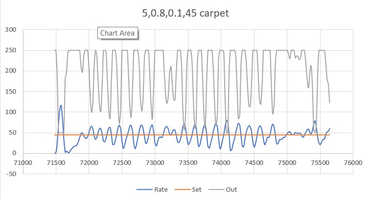
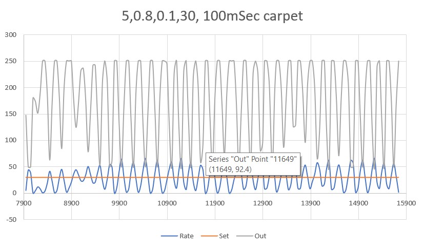
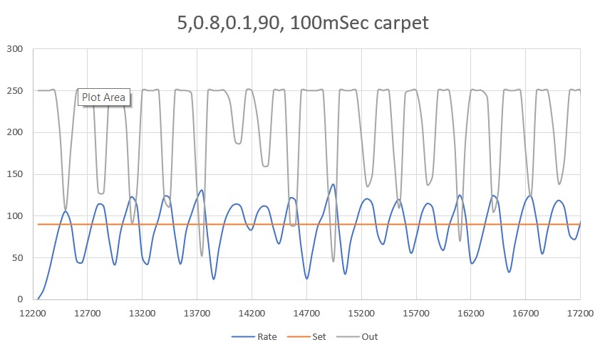
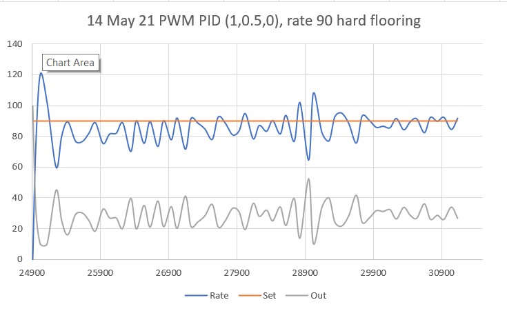
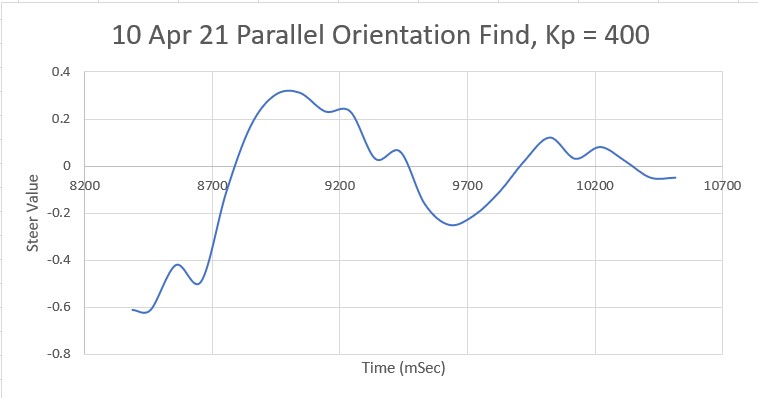
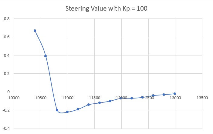
With this code, I ran a test using PID values of 300,0,0 and an offset target of 40cm. The following short video and Excel plot show the results
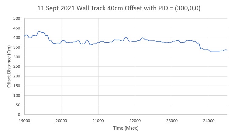
Now all I have to do is make this same trick work for both the ‘inside offset’ and ‘outside offset’ starting conditions, and then for both the left-side and right-side tracking conditions, then I can integrate the code back into the main robot operating system.
18 September 2021 Update:
After getting the left-side tracking working reasonably well, I started working on right-side tracking, and discovered that what worked for the left side with no problems did not work particularly well for right-side tracking. After the usual number of programming mistakes I did get right-side tracking working, albeit with a significantly different PID parameter set. For left-side tracking, PID = (300,0,0) seemed to work OK, but for right-side tracking I wound up with PID = (300,0,300). Moreover, when I tried even very small (like 10) values for the I parameter, the robot lost track after just two or three oscillations. So, for the moment it looks like (300,0,0) for the left side, and (300,0,300) for the right side. Here’s a short video showing successful right-side tracking.
And here is the ‘finished’ FourWD_WallTrackTest_V3 code:
|
1 2 3 4 5 6 7 8 9 10 11 12 13 14 15 16 17 18 19 20 21 22 23 24 25 26 27 28 29 30 31 32 33 34 35 36 37 38 39 40 41 42 43 44 45 46 47 48 49 50 51 52 53 54 55 56 57 58 59 60 61 62 63 64 65 66 67 68 69 70 71 72 73 74 75 76 77 78 79 80 81 82 83 84 85 86 87 88 89 90 91 92 93 94 95 96 97 98 99 100 101 102 103 104 105 106 107 108 109 110 111 112 113 114 115 116 117 118 119 120 121 122 123 124 125 126 127 128 129 130 131 132 133 134 135 136 137 138 139 140 141 142 143 144 145 146 147 148 149 150 151 152 153 154 155 156 157 158 159 160 161 162 163 164 165 166 167 168 169 170 171 172 173 174 175 176 177 178 179 180 181 182 183 184 185 186 187 188 189 190 191 192 193 194 195 196 197 198 199 200 201 202 203 204 205 206 207 208 209 210 211 212 213 214 215 216 217 218 219 220 221 222 223 224 225 226 227 228 229 230 231 232 233 234 235 236 237 238 239 240 241 242 243 244 245 246 247 248 249 250 251 252 253 254 255 256 257 258 259 260 261 262 263 264 265 266 267 268 269 270 271 272 273 274 275 276 277 278 279 280 281 282 283 284 285 286 287 288 289 290 291 292 293 294 295 296 297 298 299 300 301 302 303 304 305 306 307 308 309 310 311 312 313 314 315 316 317 318 319 320 321 322 323 324 325 326 327 328 329 330 331 332 333 334 335 336 337 338 339 340 341 342 343 344 345 346 347 348 349 350 351 352 353 354 355 356 357 358 359 360 361 362 363 364 365 366 367 368 369 370 371 372 373 374 375 376 377 378 379 380 381 382 383 384 385 386 387 388 389 390 391 392 393 394 395 396 397 398 399 400 401 402 403 404 405 406 407 408 409 410 411 412 413 414 415 416 417 418 419 420 421 422 423 424 425 426 427 428 429 430 431 432 433 434 435 436 437 438 439 440 441 442 443 444 445 446 447 448 449 450 451 452 453 454 455 456 457 458 459 460 461 462 463 464 465 466 467 468 469 470 471 472 473 474 475 476 477 478 479 480 481 482 483 484 485 486 487 488 489 490 491 492 493 494 495 496 497 498 499 500 501 502 503 504 505 506 507 508 509 510 511 512 513 514 515 516 517 518 519 520 521 522 523 524 525 526 527 528 529 530 531 532 533 534 535 536 537 538 539 540 541 542 543 544 545 546 547 548 549 550 551 552 553 554 555 556 557 558 559 560 561 562 563 564 565 566 567 568 569 570 571 572 573 574 575 576 577 578 579 580 581 582 583 584 585 586 587 588 589 590 591 592 593 594 595 596 597 598 599 600 601 602 603 604 605 606 607 608 609 610 611 612 613 614 615 616 617 618 619 620 621 622 623 624 625 626 627 628 629 630 631 632 633 634 635 636 637 638 639 640 641 642 643 644 645 646 647 648 649 650 651 652 653 654 655 656 657 658 659 660 661 662 663 664 665 666 667 668 669 670 671 672 673 674 675 676 677 678 679 680 681 682 683 684 685 686 687 688 689 690 691 692 693 694 695 696 697 698 699 700 701 702 703 704 705 706 707 708 709 710 711 712 713 714 715 716 717 718 719 720 721 722 723 724 725 726 727 728 729 730 731 732 733 734 735 736 737 738 739 740 741 742 743 744 745 746 747 748 749 750 751 752 753 754 755 756 757 758 759 760 761 762 763 764 765 766 767 768 769 770 771 772 773 774 775 776 777 778 779 780 781 782 783 784 785 786 787 788 789 790 791 792 793 794 795 796 797 798 799 800 801 802 803 804 805 806 807 808 809 810 811 812 813 814 815 816 817 818 819 820 821 822 823 824 825 826 827 828 829 830 831 832 833 834 835 836 837 838 839 840 841 842 843 844 845 846 847 848 849 850 851 852 853 854 855 856 857 858 859 860 861 862 863 864 865 866 867 868 869 870 871 872 873 874 875 876 877 878 879 880 881 882 883 884 885 886 887 888 889 890 891 892 893 894 895 896 897 898 899 900 901 902 903 904 905 906 907 908 909 910 911 912 913 914 915 916 917 918 919 920 921 922 923 924 925 926 927 928 929 930 931 932 933 934 935 936 937 938 939 940 941 942 943 944 945 946 947 948 949 950 951 952 953 954 955 956 957 958 959 960 961 962 963 964 965 966 967 968 969 970 971 972 973 974 975 976 977 978 979 980 981 982 983 984 985 986 987 988 989 990 991 992 993 994 995 996 997 998 999 1000 1001 1002 1003 1004 1005 1006 1007 1008 1009 1010 1011 1012 1013 1014 1015 1016 1017 1018 1019 1020 1021 1022 1023 1024 1025 1026 1027 1028 1029 1030 1031 1032 1033 1034 1035 1036 1037 1038 1039 1040 1041 1042 1043 1044 1045 1046 1047 1048 1049 1050 1051 1052 1053 1054 1055 1056 1057 1058 1059 1060 1061 1062 1063 1064 1065 1066 1067 1068 1069 1070 1071 1072 1073 1074 1075 1076 1077 1078 1079 1080 1081 1082 1083 1084 1085 1086 1087 1088 1089 1090 1091 1092 1093 1094 1095 1096 1097 1098 1099 1100 1101 1102 1103 1104 1105 1106 1107 1108 1109 1110 1111 1112 1113 1114 1115 1116 1117 1118 1119 1120 1121 1122 1123 1124 1125 1126 1127 1128 1129 1130 1131 1132 1133 1134 1135 1136 1137 1138 1139 1140 1141 1142 1143 1144 1145 1146 1147 1148 1149 1150 1151 1152 1153 1154 1155 1156 1157 1158 1159 1160 1161 1162 1163 1164 1165 1166 1167 1168 1169 1170 1171 1172 1173 1174 1175 1176 1177 1178 1179 1180 1181 1182 1183 1184 1185 1186 1187 1188 1189 1190 1191 1192 1193 1194 1195 1196 1197 1198 1199 1200 1201 1202 1203 1204 1205 1206 1207 1208 1209 1210 1211 1212 1213 1214 1215 1216 1217 1218 1219 1220 1221 1222 1223 1224 1225 1226 1227 1228 1229 1230 1231 1232 1233 1234 1235 1236 1237 1238 1239 1240 1241 1242 1243 1244 1245 1246 1247 1248 1249 1250 1251 1252 1253 1254 1255 1256 1257 1258 1259 1260 1261 1262 1263 1264 1265 1266 1267 1268 1269 1270 1271 1272 1273 1274 1275 1276 1277 1278 1279 1280 1281 1282 1283 1284 1285 1286 1287 1288 1289 1290 1291 1292 1293 1294 1295 1296 1297 1298 1299 1300 1301 1302 1303 1304 1305 1306 1307 1308 1309 1310 1311 1312 1313 1314 1315 1316 1317 1318 1319 1320 1321 1322 1323 1324 1325 1326 1327 1328 1329 1330 1331 1332 1333 1334 1335 1336 1337 1338 1339 1340 1341 1342 1343 1344 1345 1346 1347 1348 1349 1350 1351 1352 1353 1354 1355 1356 1357 1358 1359 1360 1361 1362 1363 1364 1365 1366 1367 1368 1369 1370 1371 1372 1373 1374 1375 1376 1377 1378 1379 1380 1381 1382 1383 1384 1385 1386 1387 1388 1389 1390 1391 1392 1393 1394 1395 1396 1397 1398 1399 1400 1401 1402 1403 1404 1405 1406 1407 1408 1409 1410 1411 1412 1413 1414 1415 1416 1417 1418 1419 1420 1421 1422 1423 1424 1425 1426 1427 1428 1429 1430 1431 1432 1433 1434 1435 1436 1437 1438 1439 1440 1441 1442 1443 1444 1445 1446 1447 1448 1449 1450 1451 1452 1453 1454 1455 1456 1457 1458 1459 1460 1461 1462 1463 1464 1465 1466 1467 1468 1469 1470 1471 1472 1473 1474 1475 1476 1477 1478 1479 1480 1481 1482 1483 1484 1485 1486 1487 1488 1489 1490 1491 1492 1493 1494 1495 1496 1497 1498 1499 1500 1501 1502 1503 1504 1505 1506 1507 1508 1509 1510 1511 1512 1513 1514 1515 1516 1517 1518 1519 1520 1521 1522 1523 1524 1525 1526 1527 1528 1529 1530 1531 1532 1533 1534 1535 1536 1537 1538 1539 1540 1541 1542 1543 1544 1545 1546 1547 1548 1549 1550 1551 1552 1553 1554 1555 1556 1557 1558 1559 1560 1561 1562 1563 1564 1565 1566 1567 1568 1569 1570 1571 1572 1573 1574 1575 1576 1577 1578 1579 1580 1581 1582 1583 1584 1585 1586 1587 1588 1589 1590 1591 1592 1593 1594 1595 1596 1597 1598 1599 1600 1601 1602 1603 1604 1605 1606 1607 1608 1609 1610 1611 1612 1613 1614 1615 1616 1617 1618 1619 1620 1621 1622 1623 1624 1625 1626 1627 1628 1629 1630 1631 1632 1633 1634 1635 1636 1637 1638 1639 1640 1641 1642 1643 1644 1645 1646 1647 1648 1649 1650 1651 1652 1653 1654 1655 1656 1657 1658 1659 1660 1661 1662 1663 1664 1665 1666 1667 1668 1669 1670 1671 1672 1673 1674 1675 1676 1677 1678 1679 1680 1681 1682 1683 1684 1685 1686 1687 1688 1689 1690 1691 1692 1693 1694 1695 1696 1697 1698 1699 1700 1701 1702 1703 1704 1705 1706 1707 1708 1709 1710 1711 1712 1713 1714 1715 1716 1717 1718 1719 1720 1721 1722 1723 1724 1725 1726 1727 1728 1729 1730 1731 1732 1733 1734 1735 1736 1737 1738 1739 1740 1741 1742 1743 1744 1745 1746 1747 1748 1749 1750 1751 1752 1753 1754 1755 1756 1757 1758 1759 1760 1761 1762 1763 1764 1765 1766 1767 1768 1769 1770 1771 1772 1773 1774 1775 1776 1777 1778 1779 1780 1781 1782 1783 1784 1785 1786 1787 1788 1789 1790 1791 1792 1793 1794 1795 1796 1797 1798 1799 1800 1801 1802 1803 1804 1805 1806 1807 1808 1809 1810 1811 1812 1813 1814 1815 1816 1817 1818 1819 1820 1821 1822 1823 1824 1825 1826 1827 1828 1829 1830 1831 1832 1833 1834 1835 1836 1837 1838 1839 1840 1841 1842 1843 1844 1845 1846 1847 1848 1849 1850 1851 1852 1853 1854 1855 1856 1857 1858 1859 1860 1861 1862 1863 1864 1865 1866 1867 1868 1869 1870 1871 1872 1873 1874 1875 1876 1877 1878 1879 1880 1881 1882 1883 1884 1885 1886 1887 1888 1889 1890 1891 1892 1893 1894 1895 1896 1897 1898 1899 1900 1901 1902 1903 1904 1905 1906 1907 1908 1909 1910 1911 1912 1913 1914 1915 1916 1917 1918 1919 1920 1921 1922 1923 1924 1925 1926 1927 1928 1929 1930 1931 1932 1933 1934 1935 1936 1937 1938 1939 1940 1941 1942 1943 1944 1945 1946 1947 1948 1949 1950 1951 1952 1953 1954 1955 1956 1957 1958 1959 1960 1961 1962 1963 1964 1965 1966 1967 1968 1969 1970 1971 1972 1973 1974 1975 1976 1977 1978 1979 1980 1981 1982 1983 1984 1985 1986 1987 1988 1989 1990 1991 1992 1993 1994 1995 1996 1997 1998 1999 2000 2001 2002 2003 2004 2005 2006 2007 2008 2009 2010 2011 2012 2013 2014 2015 2016 2017 2018 2019 2020 2021 2022 2023 2024 2025 2026 2027 2028 2029 2030 2031 2032 2033 2034 2035 2036 2037 2038 2039 2040 2041 2042 2043 2044 2045 2046 2047 2048 2049 2050 2051 2052 2053 2054 2055 2056 2057 2058 2059 2060 2061 2062 2063 2064 2065 2066 2067 2068 2069 2070 2071 2072 2073 2074 2075 2076 2077 2078 2079 2080 2081 2082 2083 2084 2085 2086 2087 2088 2089 2090 2091 2092 2093 2094 2095 2096 2097 2098 2099 2100 2101 2102 2103 2104 2105 2106 2107 2108 2109 2110 2111 2112 2113 2114 2115 2116 2117 2118 2119 2120 2121 2122 2123 2124 2125 2126 2127 2128 2129 2130 2131 2132 2133 2134 2135 2136 2137 2138 2139 2140 2141 2142 2143 2144 2145 2146 2147 2148 2149 2150 2151 2152 2153 2154 2155 2156 2157 2158 2159 2160 2161 2162 2163 2164 2165 2166 2167 2168 2169 2170 2171 2172 2173 2174 2175 2176 2177 2178 2179 2180 2181 2182 2183 2184 2185 2186 2187 2188 2189 2190 2191 2192 2193 2194 2195 2196 2197 2198 2199 2200 2201 2202 2203 2204 2205 2206 2207 2208 2209 2210 2211 2212 2213 2214 2215 2216 2217 2218 2219 2220 2221 2222 2223 2224 2225 2226 2227 2228 2229 2230 2231 2232 2233 2234 2235 2236 2237 2238 2239 2240 2241 2242 2243 2244 2245 2246 2247 2248 2249 2250 2251 2252 2253 2254 2255 2256 2257 2258 2259 2260 2261 2262 2263 2264 2265 2266 2267 2268 2269 2270 2271 2272 2273 2274 2275 2276 2277 2278 2279 2280 2281 2282 2283 2284 2285 2286 2287 2288 2289 2290 2291 2292 2293 2294 2295 2296 2297 2298 2299 2300 2301 2302 2303 2304 2305 2306 2307 2308 2309 2310 2311 2312 2313 2314 2315 2316 2317 2318 2319 2320 2321 2322 2323 2324 2325 2326 2327 2328 2329 2330 2331 2332 2333 2334 2335 2336 2337 2338 2339 2340 2341 2342 2343 2344 2345 2346 2347 2348 2349 2350 2351 2352 2353 2354 2355 2356 2357 2358 2359 2360 2361 2362 2363 2364 2365 2366 2367 2368 2369 2370 2371 2372 2373 2374 2375 2376 2377 2378 2379 2380 2381 2382 2383 2384 2385 2386 2387 2388 2389 2390 2391 2392 2393 2394 2395 2396 2397 2398 2399 2400 2401 2402 2403 2404 2405 2406 2407 2408 2409 2410 2411 2412 2413 2414 2415 |
/* Name: FourWD_WallTrackTest_V3.ino Created: 9/3/2021 6:41:37 PM Author: FRANKNEWXPS15\Frank */ /* Name: FourWD_WallTrackTest_V2.ino Created: 8/7/2021 2:23:38 PM Author: FRANKNEWXPS15\Frank */ #pragma region INCLUDES #include <elapsedMillis.h> #include <PrintEx.h> //allows printf-style printout syntax #include "MPU6050_6Axis_MotionApps_V6_12.h" //changed to this version 10/05/19 #include "I2Cdev.h" //this includes Wire.h #include "I2C_Anything.h" //needed for sending float data over I2C #include <PID_v2.h> //moved here 02/09/19 #include <MemoryFree.h>; #pragma endregion Includes #pragma region DEFINES #define MPU6050_I2C_ADDR 0x68 //08/09/21 now using default 0x68 addr, since RTC has been removed //#define DISTANCES_ONLY //added 11/14/18 to just display distances in infinite loop //#define NO_MOTORS //07/18/21 debug //#define NO_LIDAR //#define MPU6050_CCW_INCREASES_YAWVAL //added 12/05/19 #pragma endregion DEFINES #pragma region PRE_SETUP StreamEx mySerial = Serial; //added 03/18/18 for printf-style printing MPU6050 mpu(MPU6050_I2C_ADDR); //06/23/18 chg to AD0 high addr, using INT connected to Mega pin 2 (INT0) volatile int frontdistval = 0; //10/10/20 chg to volatile volatile double frontvar = 0; //08/11/20 now updated in timer1 ISR const int MAX_FRONT_DISTANCE_CM = 400; const int FRONT_DIST_AVG_WINDOW_SIZE = 3; //moved here & renamed 04/28/19 const int FRONT_DIST_ARRAY_SIZE = 50; //11/22/20 doubled to acct for 10Hz update rate uint16_t aFrontDist[FRONT_DIST_ARRAY_SIZE]; //04/18/19 rev to use uint16_t vs byte //11/03/18 added for new incremental variance calc double Front_Dist_PrevVar = 0; double Front_Dist_PrevVMean = 0; #pragma region MOTOR_PINS //09/11/20 Now using two Adafruit DRV8871 drivers for all 4 motors const int In1_Left = 10; const int In2_Left = 11; const int In1_Right = 8; const int In2_Right = 9; #pragma endregion Motor Pin Assignments #pragma region MISC_PIN_ASSIGNMENTS const int RED_LASER_DIODE_PIN = 7; const int LIDAR_MODE_PIN = 4; //mvd here 01/10/18 const int BATT_MON_PIN = A1;//BATT Monitor and IR Detector pin assignments added 01/30/17 #pragma endregion MISC_PIN_ASSIGNMENTS #pragma region MOTOR_PARAMETERS //drive wheel speed parameters const int MOTOR_SPEED_FULL = 200; //range is 0-255 const int MOTOR_SPEED_MAX = 255; //range is 0-255 const int MOTOR_SPEED_HALF = 127; //range is 0-255 const int MOTOR_SPEED_QTR = 75; //added 09/25/20 const int MOTOR_SPEED_LOW = 50; //added 01/22/15 const int MOTOR_SPEED_OFF = 0; //range is 0-255 //drive wheel direction constants const boolean FWD_DIR = true; const boolean REV_DIR = !FWD_DIR; const bool TURNDIR_CCW = true; const bool TURNDIR_CW = false; //Motor direction variables boolean bLeftMotorDirIsFwd = true; boolean bRightMotorDirIsFwd = true; bool bIsForwardDir = true; //default is foward direction #pragma endregion Motor Parameters #pragma region HEADING_AND_RATE_BASED_TURN_PARAMETERS elapsedMillis MsecSinceLastTurnRateUpdate; const int MAX_PULSE_WIDTH_MSEC = 100; const int MIN_PULSE_WIDTH_MSEC = 0; const int MAX_SPIN_MOTOR_SPEED = 250; const int MIN_SPIN_MOTOR_SPEED = 50; //const int TURN_RATE_UPDATE_INTERVAL_MSEC = 30; //const int TURN_RATE_UPDATE_INTERVAL_MSEC = 60; const int TURN_RATE_UPDATE_INTERVAL_MSEC = 100; double Prev_HdgDeg = 0; float tgt_deg; float timeout_sec; //05/31/21 latest & greatest PID values double TurnRate_Kp = 5.0; double TurnRate_Ki = 1; //double TurnRate_Kd = 0.5; //double TurnRate_Kd = 1.5; double TurnRate_Kd = 2.5; double TurnRatePIDSetPointDPS, TurnRatePIDOutput; double TurnRatePIDInput = 15.f; PID TurnRatePID(&TurnRatePIDInput, &TurnRatePIDOutput, &TurnRatePIDSetPointDPS, TurnRate_Kp, TurnRate_Ki, TurnRate_Kd, DIRECT); const float HDG_NEAR_MATCH_VAL = 0.8; //slow the turn down here const float HDG_FULL_MATCH_VAL = 0.99; //stop the turn here //rev 05/17/20 const float HDG_MIN_MATCH_VAL = 0.6; //added 09/08/18: don't start checking slope until turn is well started #pragma endregion HEADING_AND_RATE_BASED_TURN_PARAMETERS #pragma region MPU6050_SUPPORT uint8_t mpuIntStatus; // holds actual interrupt status byte from MPU. Used in Homer's Overflow routine uint8_t devStatus; // return status after each device operation (0 = success, !0 = error) uint16_t packetSize; // expected DMP packet size (default is 42 bytes) uint16_t fifoCount; // count of all bytes currently in FIFO uint8_t fifoBuffer[64]; // FIFO storage buffer // orientation/motion vars Quaternion q; // [w, x, y, z] quaternion container VectorInt16 aa; // [x, y, z] accel sensor measurements VectorInt16 aaReal; // [x, y, z] gravity-free accel sensor measurements VectorInt16 aaWorld; // [x, y, z] world-frame accel sensor measurements VectorFloat gravity; // [x, y, z] gravity vector float euler[3]; // [psi, theta, phi] Euler angle container float ypr[3]; // [yaw, pitch, roll] yaw/pitch/roll container and gravity vector int GetPacketLoopCount = 0; int OuterGetPacketLoopCount = 0; //MPU6050 status flags bool bMPU6050Ready = true; bool dmpReady = false; // set true if DMP init was successful volatile float IMUHdgValDeg = 0; //updated by UpdateIMUHdgValDeg()//11/02/20 now updated in ISR bool bFirstTime = true; #pragma endregion MPU6050 Support #pragma region WALL_FOLLOW_SUPPORT const int WALL_OFFSET_TRACK_Kp = 100; const int WALL_OFFSET_TRACK_Ki = 0; const int WALL_OFFSET_TRACK_Kd = 0; //const double WALL_OFFSET_TRACK_SETPOINT_LIMIT = 0.3; //const double WALL_OFFSET_TRACK_SETPOINT_LIMIT = 0.4; //const double WALL_OFFSET_TRACK_SETPOINT_LIMIT = 0.5; //const double WALL_OFFSET_TRACK_SETPOINT_LIMIT = 0.15; const double WALL_OFFSET_TRACK_SETPOINT_LIMIT = 0.25; double WallTrackSteerVal, WallTrackOutput, WallTrackSetPoint; const int CHG_CONNECT_LED_PIN = 50; //12/16/20 added for debug //const int WALL_OFFSET_TGTDIST_CM = 30; const int WALL_OFFSET_TGTDIST_CM = 40; double LeftSteeringVal, RightSteeringVal; //added 08/06/20 const int WALL_TRACK_UPDATE_INTERVAL_MSEC = 50; //const int WALL_TRACK_UPDATE_INTERVAL_MSEC = 30; const int WALL_OFFSET_APPR_ANGLE_MINDEG = 30;//added 09/08/21 #pragma endregion WALL_FOLLOW_SUPPORT #pragma region VL53L0X LIDAR SUPPORT //VL53L0X Sensor data values //11/05/20 revised to make all volatile volatile int Lidar_RightFront; volatile int Lidar_RightCenter; volatile int Lidar_RightRear; volatile int Lidar_LeftFront; volatile int Lidar_LeftCenter; volatile int Lidar_LeftRear; volatile int Lidar_Rear; //added 10/24/20 bool bVL53L0X_TeensyReady = false; //11/10/20 added to prevent bad data reads during Teensy setup() enum VL53L0X_REQUEST { VL53L0X_READYCHECK, //added 11/10/20 to prevent bad reads during Teensy setup() VL53L0X_CENTERS_ONLY, VL53L0X_RIGHT, VL53L0X_LEFT, VL53L0X_ALL, //added 08/06/20, replaced VL53L0X_BOTH 10/31/20 VL53L0X_REAR_ONLY //added 10/24/20 }; const int VL53L0X_I2C_SLAVE_ADDRESS = 0x20; ////Teensy 3.5 VL53L0X ToF LIDAR controller #pragma endregion VL53L0X LIDAR SUPPORT #pragma region TIMER_ISR #define TIMER_INT_OUTPUT_PIN 53 //scope monitor pin bool GetRequestedVL53l0xValues(VL53L0X_REQUEST which); volatile bool bTimeForNavUpdate = false; const int TIMER5_INTERVAL_MSEC = 100; //05/15/21 added to eliminate magic number int GetFrontDistCm(); ISR(TIMER5_COMPA_vect) //timer5 interrupt 5Hz { digitalWrite(TIMER_INT_OUTPUT_PIN, HIGH);//so I can monitor interrupt timing delayMicroseconds(30); //leave in - so can see even with NO_STUCK defined bTimeForNavUpdate = true; //11/2/20 have to re-enable interrupts for I2C comms to work interrupts(); GetRequestedVL53l0xValues(VL53L0X_ALL); //11/2/20 update all distances every 100mSec noInterrupts(); frontdistval = GetFrontDistCm(); digitalWrite(TIMER_INT_OUTPUT_PIN, LOW);//so I can monitor interrupt timing } #pragma endregion TIMER_ISR #pragma endregion PRE_SETUP #pragma region BATTCONSTS //03/10/15 added for battery charge level monitoring //const int LOW_BATT_THRESH_VOLTS = 7.4; //50% chg per http://batteryuniversity.com/learn/article/lithium_based_batteries //const int LOW_BATT_THRESH_VOLTS = 8.4; //07/10/20 temp debug settingr//50% chg per http://batteryuniversity.com/learn/article/lithium_based_batteries const float LOW_BATT_THRESH_VOLTS = 8.4; //12/18/20 chg to float to fix bug const int MAX_AD_VALUE = 1023; //const long BATT_CHG_TIMEOUT_SEC = 36000; //10 HRS const long BATT_CHG_TIMEOUT_SEC = 3600; //12/28/20 for test only const float DEAD_BATT_THRESH_VOLTS = 6; //added 01/24/17 const float FULL_BATT_VOLTS = 8.4; //added 03/17/18. Chg to 8.4 03/05/20 const int MINIMUM_CHARGE_TIME_SEC = 10; //added 04/01/18 const float VOLTAGE_TO_CURRENT_RATIO = 0.75f; //Volts/Amp rev 03/01/19. Used for both 'Total' and 'Run' sensors const float FULL_BATT_CURRENT_THRESHOLD = 0.5; //amps chg to 0.5A 03/02/19 per https://www.fpaynter.com/2019/03/better-battery-charging-for-wall-e2/ const int CURRENT_AVERAGE_NUMBER = 10; //added 03/01/19 const int VOLTS_AVERAGE_NUMBER = 5; //added 03/01/19 const int IR_HOMING_TELEMETRY_SPACING_MSEC = 200; //added 04/23/20 const float ZENER_VOLTAGE_OFFSET = 5.84; //measured zener voltage const float ADC_REF_VOLTS = 3.3; //03/27/18 now using analogReference(EXTERNAL) with Teensy 3.3V connected to AREF #pragma endregion BATTCONST void setup() { Serial.begin(115200); #pragma region MPU6050 mySerial.printf("\nChecking for MPU6050 IMU at I2C Addr 0x%x\n", MPU6050_I2C_ADDR); mpu.initialize(); // verify connection Serial.println(mpu.testConnection() ? F("MPU6050 connection successful") : F("MPU6050 connection failed")); float StartSec = 0; //used to time MPU6050 init Serial.println(F("Initializing DMP...")); devStatus = mpu.dmpInitialize(); // make sure it worked (returns 0 if successful) if (devStatus == 0) { // turn on the DMP, now that it's ready Serial.println(F("Enabling DMP...")); mpu.setDMPEnabled(true); // set our DMP Ready flag so the main loop() function knows it's okay to use it Serial.println(F("DMP ready! Waiting for MPU6050 drift rate to settle...")); dmpReady = true; // get expected DMP packet size for later comparison packetSize = mpu.dmpGetFIFOPacketSize(); mySerial.printf("Just after MPU6050 Init\n"); mySerial.printf("Calibrating...\n"); mpu.CalibrateGyro(); //using default value of 15 mySerial.printf("Retrieving Calibration Values\n\n"); mpu.PrintActiveOffsets(); //loop heading display until stabilized mySerial.printf("\nMsec\tHdg\n"); UpdateIMUHdgValDeg(); Prev_HdgDeg = IMUHdgValDeg; delay(100); UpdateIMUHdgValDeg(); mySerial.printf("%lu\t%2.3f\t%2.3f\n", millis(), IMUHdgValDeg, Prev_HdgDeg); while (abs(IMUHdgValDeg - Prev_HdgDeg) > 0.1f) { mySerial.printf("%lu\t%2.3f\n", millis(), IMUHdgValDeg); Prev_HdgDeg = IMUHdgValDeg; delay(100); UpdateIMUHdgValDeg(); } StartSec = millis() / 1000.f; mySerial.printf("MPU6050 Ready at %2.2f Sec with delta = %2.3f\n", StartSec, IMUHdgValDeg - Prev_HdgDeg); bMPU6050Ready = true; delay(1000); } else //MPU6050 Init failed for some reason { // ERROR! // 1 = initial memory load failed // 2 = DMP configuration updates failed // (if it's going to break, usually the code will be 1) Serial.print(F("DMP Initialization failed (code ")); Serial.print(devStatus); Serial.println(F(")")); //08/29/21 print out battery voltage on failure float batV = GetBattVoltage(); mySerial.printf("Battery Voltage = %2.2f\n", batV); bMPU6050Ready = false; } #pragma endregion MPU6050 #pragma region PIN_INITIALIZATION pinMode(LIDAR_MODE_PIN, INPUT); // Set LIDAR input monitor pin #pragma endregion PIN_INITIALIZATION //#pragma region TIMER_INTERRUPT // //09/18/20 can't use Timer1 cuz doing so conflicts with PWM on pins 10-12 // cli();//stop interrupts // TCCR5A = 0;// set entire TCCR5A register to 0 // TCCR5B = 0;// same for TCCR5B // TCNT5 = 0;//initialize counter value to 0 // // // 06/15/21 rewritten to use defined interval constant rather than magic number // //10/11/20 chg timer interval to 10Hz vs 5 // //OCR5A = 1562;// = (16*10^6) / (10*1024) - 1 (must be <65536) // int ocr5a = (16 * 1e6) / ((1000 / TIMER5_INTERVAL_MSEC) * 1024) - 1; // mySerial.printf("ocr5a = %d\n", ocr5a); // OCR5A = ocr5a; // TCCR5B |= (1 << WGM52);// turn on CTC mode // TCCR5B |= (1 << CS52) | (1 << CS50);// Set CS10 and CS12 bits for 1024 prescaler // TIMSK5 |= (1 << OCIE5A);// enable timer compare interrupt // sei();//allow interrupts // pinMode(TIMER_INT_OUTPUT_PIN, OUTPUT); //#pragma endregion TIMER_INTERRUPT // // //02/08/21 mvd below ISR enable so this section can use ISR-generated VL53L0X distances #pragma region VL53L0X_TEENSY mySerial.printf("Checking for Teensy 3.5 VL53L0X Controller at I2C addr 0x%x\n", VL53L0X_I2C_SLAVE_ADDRESS); while (!bVL53L0X_TeensyReady) { Wire.beginTransmission(VL53L0X_I2C_SLAVE_ADDRESS); bVL53L0X_TeensyReady = (Wire.endTransmission() == 0); //mySerial.printf("%lu: VL53L0X Teensy Not Avail...\n", millis()); delay(100); } mySerial.printf("Teensy available at %lu with bVL53L0X_TeensyReady = %d. Waiting for Teensy setup() to finish\n", millis(), bVL53L0X_TeensyReady); WaitForVL53L0XTeensy(); //mySerial.printf("VL53L0X Teensy Ready at %lu\n\n", millis()); #pragma endregion VL53L0X_TEENSY mySerial.printf("Just after WaitForVL53L0XTeensy();\n"); //11/14/18 added this section for distance printout only //08/06/20 revised for VL53L0X support #ifdef DISTANCES_ONLY //TIMSK5 = 0; digitalWrite(RED_LASER_DIODE_PIN, HIGH); //enable the front laser dot mySerial.printf("\n------------ DISTANCES ONLY MODE!!! -----------------\n\n"); int i = 0; //added 09/20/20 for in-line header display mySerial.printf("Msec\tLFront\tLCenter\tLRear\tRFront\tRCenter\tRRear\tFront\tRear\n"); while (true) { //if (bTimeForNavUpdate) //{ // bTimeForNavUpdate = false; //09/20/20 re-display the column headers //if (++i % 20 == 0) //{ // mySerial.printf("\nMsec\tLFront\tLCenter\tLRear\tRFront\tRCenter\tRRear\tFront\tRear\n"); //} //commented out 02/02/21 - now done in ISR GetRequestedVL53l0xValues(VL53L0X_ALL); frontdistval = GetFrontDistCm(); mySerial.printf("%lu\t%d\t%d\t%d\t%d\t%d\t%d\t%d\t%d\n", millis(), Lidar_LeftFront, Lidar_LeftCenter, Lidar_LeftRear, Lidar_RightFront, Lidar_RightCenter, Lidar_RightRear, frontdistval, Lidar_Rear); //} delay(50); } //TIMSK5 |= (1 << OCIE5A);// enable timer compare interrupt #endif // DISTANCES_ONLY #pragma region L/R/FRONT DISTANCE ARRAYS //09/20/20 have to do this for parallel finding to go the right way Serial.println(F("Initializing Left, Right, Front Distance Arrays...")); #ifndef NO_PINGS //03/30/21 moved FrontDistArray init ahead of left/right dist init to prevent inadvertent 'stuck' detection Serial.println(F("Initializing Front Distance Array")); InitFrontDistArray(); //08/12/20 code extracted to fcn so can call elsewhere //Serial.println(F("Updating Left\tRight Distance Arrays")); //for (size_t i = 0; i < LR_DIST_ARRAY_SIZE; i++) //{ // delay(100); //ensure enough time for ISR to update distances // mySerial.printf("%d\t%d\n", Lidar_LeftCenter, Lidar_RightCenter); // UpdateLRDistanceArrays(Lidar_LeftCenter, Lidar_RightCenter); //} //Serial.println(F("Updating Rear Distance Arrays")); //InitRearDistArray(); //mySerial.printf("Initial rear prev_mean, prev_var = %2.2f, %2.2f\n", // Rear_Dist_PrevMean, Rear_Dist_PrevVar); #else Serial.println(F("Distance Sensors Disabled")); #endif // NO_PINGS #pragma endregion L/R/FRONT DISTANCE ARRAYS #pragma region WALL_TRACK_TEST //mySerial.printf("End of test - Stopping!\n"); ////while (true) ////{ //// CheckForUserInput(); ////} //StopBothMotors(); //Serial.println(F("Setting Kp value")); //const int bufflen = 80; //char buff[bufflen]; //memset(buff, 0, bufflen); float OffsetCm; float Kp, Ki, Kd; //const char s[2] = ","; //char* token; ////consume CR/LF chars //while (Serial.available() > 0) //{ // int byte = Serial.read(); // mySerial.printf("consumed %d\n", byte); //} //while (!Serial.available()) //{ //} //Serial.readBytes(buff, bufflen); //mySerial.printf("%s\n", buff); ///* extract Kp */ //token = strtok(buff, s); //Kp = atof(token); ///* extract Ki */ //token = strtok(NULL, s); //Ki = atof(token); ///* extract Kd */ //token = strtok(NULL, s); //Kd = atof(token); ///* extract Offset in cm */ //token = strtok(NULL, s); //OffsetCm = atof(token); //mySerial.printf("Kp,Ki,Kd,OffsetCm = %2.2f, %2.2f, %2.2f, %2.2f\n", // Kp, Ki, Kd, OffsetCm);5 //Kp = 300; //Kp = 500; //Kp = 700; //Kp = 500; //Kp = 400; Kp = 300; Ki = 0; //Ki = 10; //Kd = 0; //Kd = 100; //Kd = 200; Kd = 300; OffsetCm = 40; //TrackLeftWallOffset(Kp, Ki, Kd, OffsetCm); //TrackLeftWallOffset(1, 1, 1, 1); //09/05/21 params not used TrackRightWallOffset(Kp, Ki, Kd, OffsetCm); // //mySerial.printf("Rdist\tCdist\tFdist\tsteer\toffang\n"); // //while (true) // //{ // // //double offangdeg = GetSteeringAngle(Lidar_LeftCenter / 10, LeftSteeringVal); // // double offangdeg = GetSteeringAngle(LeftSteeringVal); //06/25/21 chg to mm vs cm // // mySerial.printf("%d\t%d\t%d\t%2.4f\t%2.2f\n", Lidar_LeftRear, Lidar_LeftCenter, Lidar_LeftFront, LeftSteeringVal, offangdeg); // // delay(1000); // //} #pragma endregion WALL_TRACK_TEST //mySerial.printf("Msec\tHdg\n"); //RunBothMotors(true, MOTOR_SPEED_HALF, MOTOR_SPEED_HALF); } void loop() { int turndeg = 45; mySerial.printf("CCW turn, %d deg\n", turndeg); //SpinTurn(true, turndeg, 45); //delay(1000); SpinTurn(true, turndeg, 30); //ShowMultipleHeadingMeasurements(50); StopBothMotors(); delay(500); //mySerial.printf("CW turn, %d deg\n", turndeg); //SpinTurn(false, turndeg, 45); //delay(1000); SpinTurn(false, turndeg, 30); //ShowMultipleHeadingMeasurements(50); StopBothMotors(); delay(500); turndeg = 90; //mySerial.printf("CCW turn, %d deg\n", turndeg); //SpinTurn(true, turndeg, 45); delay(1000); SpinTurn(true, turndeg, 30); //ShowMultipleHeadingMeasurements(50); StopBothMotors(); delay(500); //mySerial.printf("CW turn, %d deg\n", turndeg); //SpinTurn(false, turndeg, 45); delay(1000); SpinTurn(false, turndeg, 30); //ShowMultipleHeadingMeasurements(50); StopBothMotors(); delay(500); //mySerial.printf("Done with turning tests. Free memory = %d\n", freeMemory()); } #pragma region VL53L0X_SUPPORT bool GetRequestedVL53l0xValues(VL53L0X_REQUEST which) { //Purpose: Obtain VL53L0X ToF sensor data from Teensy sensor handler //Inputs: // which = VL53L0X_REQUEST value denoting which combination of value to retrieve // VL53L0X_CENTERS_ONLY -> Just the left/right center sensor values // VL53L0X_RIGHT -> All three right sensor values, in front/center/rear order // VL53L0X_LEFT -> All three left sensor values, in front/center/rear order // VL53L0X_ALL -> All seven sensor values, in left/right front/center/rear/rear order // VL53L0X_REAR_ONLY -> added 10/24/20 Just the rear sensor reading //Outputs: // Requested sensor values, obtained via I2C from the VL53L0X sensor handler // Returns TRUE if data retrieval successful, otherwise FALSE //Plan: // Step1: Send request to VL53L0X handler // Step2: get the requested data //Notes: // Copied from FourWD_WallE2_V4.ino's IsIRBeamAvail() and adapted // 08/05/20 added a VL53L0X_ALL request type // 01/24/21 added error detection/reporting //Step1: Send request to VL53L0X handler //DEBUG!! //mySerial.printf("Sending %d to slave\n", which); //DEBUG!! //mySerial.printf("In GetRequestedVL53l0xValues(%d)\n", (int)which); Wire.beginTransmission(VL53L0X_I2C_SLAVE_ADDRESS); I2C_writeAnything((uint8_t)which); Wire.endTransmission(); //Step2: get the requested data int readResult = 0; int data_size = 0; switch (which) { case VL53L0X_READYCHECK: //11/10/20 added to prevent bad reads during Teensy setup() Wire.requestFrom(VL53L0X_I2C_SLAVE_ADDRESS, (int)(sizeof(bVL53L0X_TeensyReady))); readResult = I2C_readAnything(bVL53L0X_TeensyReady); break; case VL53L0X_CENTERS_ONLY: //just two data values needed here data_size = 2 * sizeof(int); Wire.requestFrom(VL53L0X_I2C_SLAVE_ADDRESS, (int)(2 * sizeof(Lidar_RightCenter))); readResult = I2C_readAnything(Lidar_RightCenter); if (readResult > 0) { I2C_readAnything(Lidar_LeftCenter); } //DEBUG!! //mySerial.printf("VL53L0X_CENTERS_ONLY case: Got LC/RC = %d, %d\n", Lidar_LeftCenter, Lidar_RightCenter); //DEBUG!! break; case VL53L0X_RIGHT: //four data values needed here data_size = 3 * sizeof(int) + sizeof(float); //DEBUG!! //mySerial.printf("data_size = %d\n", data_size); //DEBUG!! Wire.requestFrom(VL53L0X_I2C_SLAVE_ADDRESS, data_size); readResult = I2C_readAnything(Lidar_RightFront); if (readResult > 0) { readResult = I2C_readAnything(Lidar_RightCenter); } if (readResult > 0) { readResult = I2C_readAnything(Lidar_RightRear); } if (readResult > 0) { readResult = I2C_readAnything(RightSteeringVal); } //DEBUG!! //mySerial.printf("VL53L0X_RIGHT case: Got L/C/R/S = %d, %d, %d, %3.2f\n", // Lidar_RightFront, Lidar_RightCenter, Lidar_RightRear, ToFSteeringVal); //DEBUG!! break; case VL53L0X_LEFT: //four data values needed here data_size = 3 * sizeof(int) + sizeof(float); Wire.requestFrom(VL53L0X_I2C_SLAVE_ADDRESS, data_size); readResult = I2C_readAnything(Lidar_LeftFront); if (readResult > 0) { readResult = I2C_readAnything(Lidar_LeftCenter); } if (readResult > 0) { readResult = I2C_readAnything(Lidar_LeftRear); } if (readResult > 0) { readResult = I2C_readAnything(LeftSteeringVal); } //DEBUG!! //mySerial.printf("VL53L0X_RIGHT case: Got L/C/R/S = %d, %d, %d, %3.2f\n", // Lidar_LeftFront, Lidar_LeftCenter, Lidar_LeftRear, ToFSteeringVal); //DEBUG!! break; case VL53L0X_ALL: //added 08/05/20, chg to VL53L0X_ALL 10/31/20 //nine data values needed here - 7 ints and 2 floats data_size = 7 * sizeof(int) + 2 * sizeof(float); //10/31/20 added rear distance //mySerial.printf("In VL53L0X_ALL case with data_size = %d\n", data_size); Wire.requestFrom(VL53L0X_I2C_SLAVE_ADDRESS, data_size); //Lidar_LeftFront readResult = I2C_readAnything(Lidar_LeftFront); if (readResult != sizeof(Lidar_LeftFront)) { mySerial.printf("Error reading Lidar_LeftFront\n"); } //Lidar_LeftCenter readResult = I2C_readAnything(Lidar_LeftCenter); if (readResult != sizeof(Lidar_LeftCenter)) { mySerial.printf("Error reading Lidar_LeftCenter\n"); } //Lidar_LeftRear readResult = I2C_readAnything(Lidar_LeftRear); if (readResult != sizeof(Lidar_LeftRear)) { mySerial.printf("Error reading Lidar_LeftRear\n"); } //LeftSteeringVal readResult = I2C_readAnything(LeftSteeringVal); if (readResult != sizeof(LeftSteeringVal)) { mySerial.printf("Error reading LeftSteeringVal\n"); } //Lidar_RightFront readResult = I2C_readAnything(Lidar_RightFront); if (readResult != sizeof(Lidar_RightFront)) { mySerial.printf("Error reading Lidar_RightFront\n"); } //Lidar_RightCenter readResult = I2C_readAnything(Lidar_RightCenter); if (readResult != sizeof(Lidar_RightCenter)) { mySerial.printf("Error reading Lidar_RightCenter\n"); } //Lidar_RightRear readResult = I2C_readAnything(Lidar_RightRear); if (readResult != sizeof(Lidar_RightRear)) { mySerial.printf("Error reading Lidar_RightRear\n"); } //RightSteeringVal readResult = I2C_readAnything(RightSteeringVal); if (readResult != sizeof(RightSteeringVal)) { mySerial.printf("Error reading LeftSteeringVal\n"); } //Lidar_Rear readResult = I2C_readAnything(Lidar_Rear); if (readResult != sizeof(Lidar_Rear)) { mySerial.printf("Error reading Lidar_Rear\n"); } //mySerial.printf("%lu: VL53l0x - %d, %d, %d, %d, %d, %d, %d\n", // millis(), // Lidar_LeftFront, Lidar_LeftCenter, Lidar_LeftRear, // Lidar_RightFront, Lidar_RightCenter, Lidar_RightRear, // Lidar_Rear); break; //10/31/20 bugfix case VL53L0X_REAR_ONLY: //just ONE data value needed here data_size = sizeof(int); Wire.requestFrom(VL53L0X_I2C_SLAVE_ADDRESS, (int)(sizeof(Lidar_Rear))); readResult = I2C_readAnything(Lidar_Rear); //DEBUG!! //mySerial.printf("VL53L0X_REAR_ONLY case: Got Rear = %d\n", Lidar_Rear); //DEBUG!! break; default: break; } return readResult > 0; //this is true only if all reads succeed } void WaitForVL53L0XTeensy() { bVL53L0X_TeensyReady = false; while (!bVL53L0X_TeensyReady) { GetRequestedVL53l0xValues(VL53L0X_READYCHECK); //this updates bVL53L0X_TeensyReady //mySerial.printf("%lu: got %d from VL53L0X Teensy\n", millis(), bVL53L0X_TeensyReady); delay(100); } Serial.print(F("Teensy setup() finished at ")); Serial.printf("%lu mSec\n", millis()); //now try to get a VL53L0X measurement //11/08/20 rev to loop until all distance sensors provide valid data //mySerial.printf("Msec\tLFront\tLCtr\tLRear\tRFront\tRCtr\tRRear\tRear\n"); GetRequestedVL53l0xValues(VL53L0X_ALL); //09/04/21 now doing directly w/o ISR //mySerial.printf("%lu: %d\t%d\t%d\t%d\t%d\t%d\t%d\n", // millis(), Lidar_LeftFront, Lidar_LeftCenter, Lidar_LeftRear, // Lidar_RightFront, Lidar_RightCenter, Lidar_RightRear, Lidar_Rear); while (Lidar_LeftFront <= 0 || Lidar_LeftCenter <= 0 || Lidar_LeftRear <= 0 || Lidar_LeftFront <= 0 || Lidar_LeftCenter <= 0 || Lidar_LeftRear <= 0 || Lidar_Rear <= 0) { ////values updated 10 times/sec in ISR mySerial.printf("%lu: %d\t%d\t%d\t%d\t%d\t%d\t%d\n", millis(), Lidar_LeftFront, Lidar_LeftCenter, Lidar_LeftRear, Lidar_RightFront, Lidar_RightCenter, Lidar_RightRear, Lidar_Rear); delay(100); GetRequestedVL53l0xValues(VL53L0X_ALL); //09/04/21 now doing directly w/o ISR } mySerial.printf("VL53L0X Teensy Ready at %lu\n\n", millis()); } double GetSteeringAngle(double steerval) { //Purpose: Convert a steering angle into the equivalent off-parallel orientation in degrees //Inputs: // steerval = double value denoting current steering value // Notes: // 06/27/21 now steering_val/off_angle slope is a constant 0.0175 const double slopeval = 0.0175; double offparalleldeg = steerval / slopeval; //e.g. for steerval = -0.187 @ 10cm offset, returns +21deg //mySerial.printf("GetSteeringAngle(%d, %2.4f): slopeval = %2.4f, res %2.2f\n", ctrdist_cm, steerval, slopeval, offparalleldeg); return offparalleldeg; } #pragma endregion VL53L0X_SUPPORT #pragma region LIDAR_SUPPORT //11/05/15 added to get LIDAR measurement int GetFrontDistCm() { //Notes: // 12/05/15 chg to MODE line vs I2C // 01/06/16 rev to return avg of prev distances on error #ifndef NO_LIDAR unsigned long pulse_width; int LIDARdistCm; pulse_width = pulseIn(LIDAR_MODE_PIN, HIGH); // Count how long the pulse is high in microseconds LIDARdistCm = pulse_width / 10; // 10usec = 1 cm of distance for LIDAR-Lite //chk for erroneous reading if (LIDARdistCm == 0) { //replace with average of last three readings from aFrontDist int avgdist = GetAvgFrontDistCm(); mySerial.printf("%lu: Error in GetFrontDistCm() - %d replaced with %d\n", millis(), LIDARdistCm, avgdist); LIDARdistCm = avgdist; } //04/30/17 added limit detection/correction LIDARdistCm = (LIDARdistCm > 0) ? LIDARdistCm : MAX_FRONT_DISTANCE_CM; return LIDARdistCm; #else return 10; //safe number, I hope #endif } //04/25/21 rewritten to use aFrontDist[] values float GetAvgFrontDistCm() { int avgdist = 0; for (int i = 0; i < FRONT_DIST_AVG_WINDOW_SIZE; i++) { //DEBUG!! //mySerial.printf("frontdist[%d] = %d\n", FRONT_DIST_ARRAY_SIZE - 1 - i, aFrontDist[FRONT_DIST_ARRAY_SIZE - 1 - i]); //DEBUG!! avgdist += aFrontDist[FRONT_DIST_ARRAY_SIZE - 1 - i]; } //DEBUG!! //mySerial.printf("avgdisttot = %d\n", avgdist); //DEBUG!! avgdist = (int)((float)avgdist / (float)FRONT_DIST_AVG_WINDOW_SIZE); //DEBUG!! //mySerial.printf("avgdist = %d\n", avgdist); //DEBUG!! return avgdist; } //08/12/20 Extracted inline FRONT_DIST_ARRAY init code so can be called from anywhere void InitFrontDistArray() { //04/01/15 initialize 'stuck detection' arrays //06/17/20 re-wrote for better readability //to ensure var > STUCK_FRONT_VARIANCE_THRESHOLD for first FRONT_DIST_ARRAY_SIZE loops //array is initialized with sawtooth from 0 to MAX_FRONT_DISTANCE_CM int newval = 0; int bumpval = MAX_FRONT_DISTANCE_CM / FRONT_DIST_ARRAY_SIZE; bool bgoingUp = true; for (int i = 0; i < FRONT_DIST_ARRAY_SIZE; i++) { aFrontDist[i] = newval; //DEBUG!! //mySerial.printf("i = %d, newval = %d, aFrontdist[%d] = %d\n", i, newval, i, aFrontDist[i]); //DEBUG!! if (bgoingUp) { if (newval < MAX_FRONT_DISTANCE_CM - bumpval) //don't want newval > MAX_FRONT_DISTANCE_CM { newval += bumpval; } else { bgoingUp = false; } } else { if (newval > bumpval) //don't want newval < 0 { newval -= bumpval; } else { bgoingUp = true; } } } //04/19/19 init Front_Dist_PrevVMean & Front_Dist_PrevVar to mean/var respectively long sum = 0; for (int i = 0; i < FRONT_DIST_ARRAY_SIZE; i++) { sum += aFrontDist[i]; //adds in rest of values } Front_Dist_PrevVMean = (float)sum / (float)FRONT_DIST_ARRAY_SIZE; // Step2: calc new 'brute force' variance float sumsquares = 0; for (int i = 0; i < FRONT_DIST_ARRAY_SIZE; i++) { sumsquares += (aFrontDist[i] - Front_Dist_PrevVMean) * (aFrontDist[i] - Front_Dist_PrevVMean); } Front_Dist_PrevVar = sumsquares / FRONT_DIST_ARRAY_SIZE; mySerial.printf("%lu: aFrontDist Init: Front_Dist_PrevVMean = %3.2f, Front_Dist_PrevVar = %3.2f\n", millis(), Front_Dist_PrevVMean, Front_Dist_PrevVar); frontvar = Front_Dist_PrevVar; //added 03/30/21 to prevent 'stuck' at startup } #pragma endregion LIDAR_SUPPORT #pragma region MOTOR SUPPORT //09/08/20 modified for DRV8871 motor driver void MoveReverse(int leftspeednum, int rightspeednum) { //Purpose: Move in reverse direction continuously - companion to MoveAhead() //ProvEnA_Pinnce: G. Frank Paynter 09/08/18 //Inputs: // leftspeednum = integer denoting speed (0=stop, 255 = full speed) // rightspeednum = integer denoting speed (0=stop, 255 = full speed) //Outputs: both drive Motors energized with the specified speed //Plan: // Step 1: Set reverse direction for both wheels // Step 2: Run both Motors at specified speeds //Notes: // 01/22/20 now using Adafruit DRV8871 drivers //Step 1: Set reverse direction and speed for both wheels SetLeftMotorDirAndSpeed(REV_DIR, leftspeednum); SetRightMotorDirAndSpeed(REV_DIR, rightspeednum); } //09/08/20 modified for DRV8871 motor driver void MoveAhead(int leftspeednum, int rightspeednum) { //Purpose: Move ahead continuously //ProvEnA_Pinnce: G. Frank Paynter and Danny Frank 01/24/2014 //Inputs: // leftspeednum = integer denoting speed (0=stop, 255 = full speed) // rightspeednum = integer denoting speed (0=stop, 255 = full speed) //Outputs: both drive Motors energized with the specified speed //Plan: // Step 1: Set forward direction for both wheels // Step 2: Run both Motors at specified speeds //Notes: // 01/22/20 now using Adafruit DRV8871 drivers //mySerial.printf("InMoveAhead(%d,%d)\n", leftspeednum, rightspeednum); //Step 1: Set forward direction and speed for both wheels SetLeftMotorDirAndSpeed(true, leftspeednum); SetRightMotorDirAndSpeed(true, rightspeednum); } //09/08/10 modified for DRV8871 motor driver void StopLeftMotors() { analogWrite(In1_Left, MOTOR_SPEED_OFF); analogWrite(In2_Left, MOTOR_SPEED_OFF); } void StopRightMotors() { analogWrite(In1_Right, MOTOR_SPEED_OFF); analogWrite(In2_Right, MOTOR_SPEED_OFF); } //09/08/20 added bool bisFwd param for DRV8871 motor driver void RunBothMotors(bool bisFwd, int leftspeednum, int rightspeednum) { //Purpose: Run both Motors at left/rightspeednum speeds //Inputs: // speednum = speed value (0 = OFF, 255 = full speed) //Outputs: Both Motors run for timesec seconds at speednum speed //Plan: // Step 1: Apply drive to both wheels //Notes: // 01/14/15 - added left/right speed offset for straightness compensation // 01/22/15 - added code to restrict fast/slow values // 01/24/15 - revised for continuous run - no timing // 01/26/15 - speednum modifications moved to UpdateWallFollowmyMotorspeeds() // 12/07/15 - chg args from &int to int //Step 1: Apply drive to both wheels //DEBUG!! //mySerial.printf("In RunBothMotors(%s, %d,%d)\n", bisFwd? "FWD":"REV", leftspeednum, rightspeednum); //DEBUG!! SetLeftMotorDirAndSpeed(bisFwd, leftspeednum); SetRightMotorDirAndSpeed(bisFwd, rightspeednum); } void RunBothMotorsBidirectional(int leftspeed, int rightspeed) { //Purpose: Accommodate the need for independent bidirectional wheel motion //Inputs: // leftspeed - integer denoting left wheel speed. Positive value is fwd, negative is rev // rightspeed - integer denoting right wheel speed. Positive value is fwd, negative is rev //Outputs: // left/right wheel motors direction and speed set as appropriate //Plan: // Step1: Set left wheel direction and speed // Step2: Set right wheel direction and speed //Step1: Set left wheel direction and speed //DEBUG!! //mySerial.printf("In RunBothMotorsBidirectional(%d, %d)\n", leftspeed, rightspeed); if (leftspeed < 0) { SetLeftMotorDirAndSpeed(false, -leftspeed); //neg value ==> reverse } else { SetLeftMotorDirAndSpeed(true, leftspeed); //pos or zero value ==> fwd } //Step2: Set right wheel direction and speed if (rightspeed < 0) { SetRightMotorDirAndSpeed(false, -rightspeed); //neg value ==> reverse } else { SetRightMotorDirAndSpeed(true, rightspeed); //pos or zero value ==> fwd } } //09/08/20 added bool bisFwd param for DRV8871 motor driver void RunBothMotorsMsec(bool bisFwd, int timeMsec, int leftspeednum, int rightspeednum) { //Purpose: Run both Motors for timesec seconds at speednum speed //Inputs: // timesec = time in seconds to run the Motors // speednum = speed value (0 = OFF, 255 = full speed) //Outputs: Both Motors run for timesec seconds at speednum speed //Plan: // Step 1: Apply drive to both wheels // Step 2: Delay timsec seconds // Step 3: Remove drive from both wheels. //Notes: // 01/14/15 - added left/right speed offset for straightness compensation // 01/22/15 - added code to restrict fast/slow values // 11/25/15 - rev to use motor driver class object // 09/08/20 added bool bisFwd param for DRV8871 motor driver RunBothMotors(bisFwd, leftspeednum, rightspeednum); //Step 2: Delay timsec seconds delay(timeMsec); //Step3: Stop motors added 04/12/21 StopBothMotors(); } //11/25/15 added for symmetry ;-). void StopBothMotors() { StopLeftMotors(); StopRightMotors(); } void SetLeftMotorDirAndSpeed(bool bIsFwd, int speed) { //mySerial.printf("SetLeftMotorDirAndSpeed(%d,%d)\n", bIsFwd, speed); #ifndef NO_MOTORS if (bIsFwd) { digitalWrite(In1_Left, LOW); analogWrite(In2_Left, speed); //mySerial.printf("In TRUE block of SetLeftMotorDirAndSpeed(%s, %d)\n", // (bIsFwd == true) ? "true" : "false", speed); } else { //mySerial.printf("In FALSE block of SetLeftMotorDirAndSpeed(%s, %d)\n", // (bIsFwd == true) ? "true" : "false", speed); digitalWrite(In2_Left, LOW); analogWrite(In1_Left, speed); } #endif // !NO_MOTORS } void SetRightMotorDirAndSpeed(bool bIsFwd, int speed) { //mySerial.printf("In SetRightMotorDirAndSpeed(%s, %d)\n", // (bIsFwd == true) ? "true" : "false", speed); #ifndef NO_MOTORS if (bIsFwd) { //mySerial.printf("In TRUE block of SetRighttMotorDirAndSpeed(%s, %d)\n", // (bIsFwd == true) ? "true" : "false", speed); digitalWrite(In1_Right, LOW); analogWrite(In2_Right, speed); } else { //mySerial.printf("In FALSE block of SetRightMotorDirAndSpeed(%s, %d)\n", // (bIsFwd == true) ? "true" : "false", speed); digitalWrite(In2_Right, LOW); analogWrite(In1_Right, speed); } #endif // !NO_MOTORS } #pragma endregion Motor Support Functions #pragma region MPU5060 Support float UpdateIMUHdgValDeg() { //Purpose: Get latest yaw (heading) value from IMU //Inputs: None. This function should only be called after mpu.dmpPacketAvailable() returns TRUE //Outputs: // returns true if successful, otherwise false // IMUHdgValDeg updated on success //Plan: //Step1: check for overflow and reset the FIFO if it occurs. In this case, wait for new packet //Step2: read all available packets to get to latest data //Step3: update IMUHdgValDeg with latest value //Notes: // 10/08/19 changed return type to boolean // 10/08/19 no longer need mpuIntStatus // 10/21/19 completely rewritten to use Homer's algorithm // 05/05/20 changed return type to float vs bool. bool retval = false; int flag = mpu.GetCurrentFIFOPacket(fifoBuffer, packetSize); //08/01/21 now using library version if (flag != 0) //0 = error exit, 1 = normal exit, 2 = recovered from an overflow { // display Euler angles in degrees mpu.dmpGetQuaternion(&q, fifoBuffer); mpu.dmpGetGravity(&gravity, &q); mpu.dmpGetYawPitchRoll(ypr, &q, &gravity); //compute the yaw value IMUHdgValDeg = ypr[0] * 180 / M_PI; retval = true; } //return retval; return IMUHdgValDeg;//05/05/20 now returns updated value for use convenience } #pragma endregion MPU5060 Support #pragma region HDG_BASED_TURN_SUPPORT float GetHdgMatchVal(float tgt_deg, float cur_deg) { //Purpose: Compute the match ratio between two compass headings //Inputs: // tgt_deg = float representing target heading in +/-180 range // IMUHdgValDeg = float representing sensor yaw value in +/-180 deg range //Outputs: // returns result of 1 - abs(Tgt_deg - Hdg_deg)/180, all angles in 0-360 deg range //Plan: // Step1: convert both inputs to 0-360 deg range // Step2: compute match ratio //Notes: // formula from https://gis.stackexchange.com/questions/129954/comparing-compass-bearings //Step1: convert both inputs to 0-360 deg range float tgthdg = (tgt_deg < 0) ? tgt_deg + 360 : tgt_deg; float curhdg = (cur_deg < 0) ? cur_deg + 360 : cur_deg; //Step2: compute match ratio float match_ratio = 1 - abs(tgthdg - curhdg) / 180; //DEBUG!! //mySerial.printf("tgt\tcur\tmatch = %4.2f\t%4.2f\t%1.3f\n", tgthdg, curhdg, match_ratio); //DEBUG!! return abs(match_ratio); } bool SpinTurn(bool b_ccw, float numDeg, float degPersec) //04/25/21 added turn-rate arg (default = TURN_RATE_TARGET_DEGPERSEC) { //Purpose: Make a numDeg CW or CCW 'spin' turn //Inputs: // b_ccw - True if turn is to be ccw, false otherwise // numDeg - angle to be swept out in the turn // ROLLING_TURN_MAX_SEC_PER_DEG = const used to generate timeout proportional to turn deg // IMUHdgValDeg = IMU heading value updated by UpdateIMUHdgValDeg() //11/02/20 now updated in ISR // degPerSec = float value denoting desired turn rate //Plan: // Step1: Get current heading as starting point // Step2: Disable TIMER5 interrupts // Step3: Compute new target value & timeout value // Step4: Run motors until target reached, using inline PID algorithm to control turn rate // Step5: Re-enable TIMER5 interrupts //Notes: // 06/06/21 we-written to remove PID library - now uses custom 'PIDCalcs()' function // 06/06/21 added re-try for 180.00 return from IMU - could be bad value // 06/11/21 added code to correct dHdg errors due to 179/-179 transition & bad IMU values // 06/12/21 cleaned up & commented out debug code float tgt_deg; float timeout_sec; bool bDoneTurning = false; bool bTimedOut = false; bool bResult = true; //04/21/20 added so will be only one exit point //DEBUG!! mySerial.printf("In SpinTurn(%s, %2.2f, %2.2f)\n", b_ccw == TURNDIR_CCW ? "CCW" : "CW", numDeg, degPersec); //mySerial.printf("TurnRatePID started with Kp/Ki/Kd = %2.1f,%2.1f,%2.1f, SampleTime(mSec) = %d\n", //TurnRate_Kp, TurnRate_Ki, TurnRate_Kd, TURN_RATE_UPDATE_INTERVAL_MSEC); //DEBUG!! //no need to continue if the IMU isn't available if (!dmpReady) { mySerial.printf("DMP Failure - returning FALSE\n"); return false; } //Step1: Get current heading as starting point //06/06/21 it is possible for IMU to return 180.00 on failure //so try again. If it really IS 180, then //it will eventually time out and go on //08/26/21 re-wrote using 3-value array to make sure initial heading is a steady value UpdateIMUHdgValDeg(); int retries = 0; //if (IMUHdgValDeg == 180.f && retries < 5) if ((IMUHdgValDeg == 180.f || IMUHdgValDeg == 0.f) && retries < 5) { //DEBUG!! //mySerial.printf("Got 180.00 exactly from IMU - retrying...\n"); mySerial.printf("Got 180.00 or 0.00 exactly (%2.3f) from IMU - retrying %d...\n", IMUHdgValDeg, retries); //DEBUG!! UpdateIMUHdgValDeg(); retries++; delay(100); } //Step2: Compute new target value & timeout value timeout_sec = 3 * numDeg / degPersec; //05/29/21 rev to use new turn rate parmeter //05/17/20 limit timeout_sec to 1 sec or more timeout_sec = (timeout_sec < 1) ? 1.f : timeout_sec; //UpdateIMUHdgValDeg(); //12/05/19 added #define back in to manage which direction increases yaw values #ifdef MPU6050_CCW_INCREASES_YAWVAL tgt_deg = b_ccw ? IMUHdgValDeg + numDeg : IMUHdgValDeg - numDeg; #else tgt_deg = b_ccw ? IMUHdgValDeg - numDeg : IMUHdgValDeg + numDeg; #endif // MPU6050_CCW_INCREASES_YAWVAL //correct for -180/180 transition if (tgt_deg < -180) { tgt_deg += 360; } //07/29/19 bugfix if (tgt_deg > 180) { tgt_deg -= 360; } //DEBUG!! //mySerial.printf("Init hdg = %4.2f deg, Turn = %4.2f deg, tgt = %4.2f deg, timeout = %4.2f sec\n\n", // IMUHdgValDeg, numDeg, tgt_deg, timeout_sec); //DEBUG!! float curHdgMatchVal = 0; //09/08/18 added to bolster end-of-turn detection float prevHdgMatchVal = 0; float matchSlope = 0; //Step2: Disable TIMER5 interrupts TIMSK5 = 0; //disable timer compare interrupt //Step3: Run motors until target reached, using PID algorithm to control turn rate Prev_HdgDeg = IMUHdgValDeg; //06/10/21 synch Prev_HdgDeg & IMUHdgValDeg just before entering loop //DEBUG!! //mySerial.printf("Just before while() loop: hdg/prvhdg = %2.2f\t%2.2f\n\n", IMUHdgValDeg, Prev_HdgDeg); //mySerial.printf("Msec\tHdg\tPrvHdg\tDhdg\trate\tSet\terror\tKp*err\tKi*err\tKd*Din\tOutput\Match\tSlope\n"); //DEBUG!! elapsedMillis sinceLastTimeCheck = 0; elapsedMillis sinceLastComputeTime = 0; double lastError = 0; double lastInput = 0; double lastIval = 0; double lastDerror = 0; bool bFirstIMUHdg = true; while (!bDoneTurning && !bTimedOut) { //11/06/20 now just loops between PID calcs CheckForUserInput(); if (sinceLastComputeTime >= TURN_RATE_UPDATE_INTERVAL_MSEC) { sinceLastComputeTime -= TURN_RATE_UPDATE_INTERVAL_MSEC; UpdateIMUHdgValDeg(); //update IMUHdgValDeg double dHdg = IMUHdgValDeg - Prev_HdgDeg; if (dHdg > 180) { dHdg -= 360; mySerial.printf("dHdg > 180 - subtracting 360\n"); } else if (dHdg < -180) { dHdg += 360; mySerial.printf("dHdg < -180 - adding 360\n"); } //watch for turn rates that are wildly off double rate = abs(1000 * dHdg / TURN_RATE_UPDATE_INTERVAL_MSEC); //if (rate > 3 * degPersec) //{ // //DEBUG!! // mySerial.printf("hdg/prevhdg/dHdg/rate = %2.2f\t%2.2f\t%2.2f\t%2.2f, excessive rate - replacing with %2.2f\n", IMUHdgValDeg, Prev_HdgDeg, dHdg, rate, degPersec); // //DEBUG!! // rate = degPersec; //} //06/11/21 don't do calcs first time through, as Prev_HdgDeg isn't valid yet if (bFirstIMUHdg) { bFirstIMUHdg = false; Prev_HdgDeg = IMUHdgValDeg; //re-synch prev to curr hdg for next time } else { TurnRatePIDOutput = PIDCalcs(rate, degPersec, TURN_RATE_UPDATE_INTERVAL_MSEC, lastError, lastInput, lastIval, lastDerror, TurnRate_Kp, TurnRate_Ki, TurnRate_Kd); //PIDCalcs(rate, degPersec, TURN_RATE_UPDATE_INTERVAL_MSEC, lastError, lastInput, lastIval, lastDerror, TurnRate_Kp, TurnRate_Ki, TurnRate_Kd, TurnRatePIDOutput); int speed = 0; (TurnRatePIDOutput > MOTOR_SPEED_MAX) ? speed = MOTOR_SPEED_MAX : speed = (int)TurnRatePIDOutput; (TurnRatePIDOutput <= MOTOR_SPEED_LOW) ? speed = MOTOR_SPEED_LOW : speed = (int)TurnRatePIDOutput; SetLeftMotorDirAndSpeed(!b_ccw, speed); SetRightMotorDirAndSpeed(b_ccw, speed); //check for nearly there and all the way there curHdgMatchVal = GetHdgMatchVal(tgt_deg, IMUHdgValDeg); matchSlope = curHdgMatchVal - prevHdgMatchVal; //DEBUG!! //mySerial.printf("%lu\t%2.2f\t%2.2f\t%2.2f\t%2.2f\t%2.2f\t%2.2f\t%2.2f\t%2.2f\t%2.2f\t%d\t%2.2f\t%2.2f\n", // millis(), // IMUHdgValDeg, // Prev_HdgDeg, // dHdg, // rate, // degPersec, // lastError, // TurnRate_Kp * lastError, // TurnRate_Ki * lastIval, // TurnRate_Kd * lastDerror, // speed, // curHdgMatchVal, // matchSlope); //DEBUG!! Prev_HdgDeg = IMUHdgValDeg; //re-synch prev to curr hdg for next time //look for full match bDoneTurning = (curHdgMatchVal >= HDG_FULL_MATCH_VAL || (prevHdgMatchVal >= HDG_MIN_MATCH_VAL && matchSlope <= -0.01)); //have to use < vs <= as slope == 0 at start //mySerial.printf("curHdgMatchVal = %2.2f, prevHdgMatchVal = %2.2f, matchslope = %2.2f, bDoneTurning = %d\n", // curHdgMatchVal, // prevHdgMatchVal, // matchSlope, // bDoneTurning); prevHdgMatchVal = curHdgMatchVal; //07/31/21 moved below bDoneTurning chk so can use prevHdgMatchVal vs curHdgMatchVal in slope check } } // // bTimedOut = (sinceLastTimeCheck > timeout_sec * 1000); // // if (bTimedOut) // { // //DEBUG!! // mySerial.printf("timed out with yaw = %3.2f, tgt = %3.2f, and match = %1.3f\n", IMUHdgValDeg, tgt_deg, curHdgMatchVal); // //DEBUG!! // // bResult = false; // } // // if (bDoneTurning) // { // mySerial.printf("Completed turn with yaw = %3.2f, tgt = %3.2f, and match = %1.3f\n", IMUHdgValDeg, tgt_deg, curHdgMatchVal); // } } // // //DEBUG!! // //mySerial.printf("%lu: Exiting SpinTurn() at %3.2f deg\n", millis(), IMUHdgValDeg); // //DEBUG!! // ////Step4: Re-enable TIMER5 interrupts // TIMSK5 |= (1 << OCIE5A);// enable timer compare interrupt // StopBothMotors(); delay(1000); //added 04/27/21 for debug return bResult; } #pragma endregion HDG_BASED_TURN_SUPPORT #pragma region WALL_TRACK_SUPPORT void TrackLeftWallOffset(double kp, double ki, double kd, double offsetCm) { //Notes: // 06/21/21 modified to do a turn, then straight, then track 0 steer val elapsedMillis sinceLastComputeTime = 0; double lastError = 0; double lastInput = 0; double lastIval = 0; double lastDerror = 0; bool bFirstTime = true; double spinRateDPS = 30; GetRequestedVL53l0xValues(VL53L0X_LEFT); //update LeftSteeringVal mySerial.printf("\nIn TrackLeftWallOffset with Kp/Ki/Kd = %2.2f\t%2.2f\t%2.2f\n", kp, ki, kd); //06/21/21 modified to do a turn, then straight, then track 0 steer val double cutAngleDeg = WALL_OFFSET_TGTDIST_CM - (int)(Lidar_LeftCenter / 10.f);//positive inside, negative outside desired offset mySerial.printf("R/C/F dists = %d\t%d\t%d Steerval = %2.3f, CutAngle = %2.2f\n", Lidar_LeftRear, Lidar_LeftCenter, Lidar_LeftFront, LeftSteeringVal, cutAngleDeg); //07/05/21 implement 15deg min cut angle if (cutAngleDeg < 0 && abs(cutAngleDeg) < WALL_OFFSET_APPR_ANGLE_MINDEG) { mySerial.printf("(cutAngleDeg < 0 && abs(cutAngleDeg) < %d -- setting to -%d\n", WALL_OFFSET_APPR_ANGLE_MINDEG, WALL_OFFSET_APPR_ANGLE_MINDEG); cutAngleDeg = -WALL_OFFSET_APPR_ANGLE_MINDEG; } else if (cutAngleDeg > 0 && cutAngleDeg < WALL_OFFSET_APPR_ANGLE_MINDEG) { mySerial.printf("(cutAngleDeg > 0 && abs(cutAngleDeg) < %d -- setting to +%d\n", WALL_OFFSET_APPR_ANGLE_MINDEG, WALL_OFFSET_APPR_ANGLE_MINDEG); cutAngleDeg = WALL_OFFSET_APPR_ANGLE_MINDEG; } double SteerAngleDeg = GetSteeringAngle(LeftSteeringVal); mySerial.printf("R/C/F dists = %d\t%d\t%d Steerval = %2.3f, SteerAngle = %2.2f, CutAngle = %2.2f\n", Lidar_LeftRear, Lidar_LeftCenter, Lidar_LeftFront, LeftSteeringVal, SteerAngleDeg, cutAngleDeg); double adjCutAngleDeg = 0; uint16_t fudgeFactorMM = 0; //07/05/21 added so can change for inside vs outside starting condx if (cutAngleDeg > 0) //robot inside desired offset distance { if (SteerAngleDeg > cutAngleDeg) // --> SteerAngleDeg also > 0 { mySerial.printf("CutAngDeg > 0, SteerAngleDeg > cutAngleDeg\n"); SpinTurn(true, SteerAngleDeg - cutAngleDeg, spinRateDPS); // } else if (SteerAngleDeg < cutAngleDeg)// --> SteerAngleDeg could be < 0 { mySerial.printf("CutAngDeg > 0, SteerAngleDeg < cutAngleDeg\n"); if (SteerAngleDeg <= 0) //cutAngleDeg > 0, SteerAngleDeg <= 0 { mySerial.printf("CutAngDeg > 0, SteerAngleDeg < cutAngleDeg, SteerAngleDeg <= 0\n"); SpinTurn(false, cutAngleDeg - SteerAngleDeg, spinRateDPS); //null out SteerAngleDeg & then turn addnl cutAngleDeg } else //SteerAngleDeg < cutAngleDeg but still > 0 { mySerial.printf("CutAngDeg > 0, 0 < SteerAngleDeg < cutAngleDeg\n"); mySerial.printf("else\n"); SpinTurn(false, cutAngleDeg - SteerAngleDeg, spinRateDPS); //turn diff between SteerAngleDeg & cutAngleDeg } } fudgeFactorMM = -100; //07/05/21 don't need fudge factor for inside start condx } else // cutAngleDeg < 0 --> robot outside desired offset distance { if (SteerAngleDeg > cutAngleDeg) // --> SteerAngleDeg may also be > 0 { mySerial.printf("CutAngDeg < 0, SteerAngleDeg > cutAngleDeg\n"); SpinTurn(true, SteerAngleDeg - cutAngleDeg, spinRateDPS); // } else if (SteerAngleDeg < cutAngleDeg)// --> SteerAngleDeg must also be < 0 { if (SteerAngleDeg <= 0) //cutAngleDeg < 0, SteerAngleDeg <= 0 { mySerial.printf("CutAngDeg < 0, SteerAngleDeg <= 0\n"); SpinTurn(false, cutAngleDeg - SteerAngleDeg, spinRateDPS); //null out SteerAngleDeg & then turn addnl cutAngleDeg } else //SteerAngleDeg < cutAngleDeg but still > 0 { mySerial.printf("CutAngDeg < 0, 0 < SteerAngleDeg < cutAngleDeg\n"); SpinTurn(false, cutAngleDeg - SteerAngleDeg, spinRateDPS); //turn diff between SteerAngleDeg & cutAngleDeg } } fudgeFactorMM = 100; //07/05/21 need fudge factor for outside start condx } delay(1000); //adjust so offset capture occurs at correct perpendicular offset double adjfactor = cos(PI * cutAngleDeg / 180.f); int adjOffsetMM = (int)(10 * (double)WALL_OFFSET_TGTDIST_CM / adjfactor); adjOffsetMM += fudgeFactorMM; //fudge factor for distance measurements lagging behind robot's travel. mySerial.printf("\nat approach start: cut angle = %2.3f, adjfactor = %2.3f, tgt dist = %d\n", cutAngleDeg, adjfactor, adjOffsetMM); GetRequestedVL53l0xValues(VL53L0X_ALL); //added 09/05/21 long int err = Lidar_LeftFront - adjOffsetMM; //neg for inside going out, pos for outside going in long int prev_err = err; mySerial.printf("At start - err = prev_err = %ld\n", err, prev_err); SteerAngleDeg = GetSteeringAngle(LeftSteeringVal); mySerial.printf("R/C/F dists = %d\t%d\t%d Steerval = %2.3f, SteerAngle = %2.2f, CutAngle = %2.2f, err/prev_err = %li\n", Lidar_LeftRear, Lidar_LeftCenter, Lidar_LeftFront, LeftSteeringVal, SteerAngleDeg, cutAngleDeg, err); mySerial.printf("Msec\tLFront\tLCtr\tLRear\tFront\tRear\tErr\tP_err\n"); //TIMSK5 = 0; //turn off TIMER5 interrupts //09/05/21 rev to doublecheck robot position - might not need the forward motion section //while (prev_res * res > 0) //sign change makes this < 0 while (((cutAngleDeg > 0 && err < 0 ) || (cutAngleDeg <= 0 && err >= 0)) && prev_err * err > 0) //sign change makes this < 0 { prev_err = err; MoveAhead(MOTOR_SPEED_QTR, MOTOR_SPEED_QTR); //while (!bTimeForNavUpdate) //{ //} delay(100); bTimeForNavUpdate = false; frontdistval = GetFrontDistCm(); GetRequestedVL53l0xValues(VL53L0X_ALL); err = Lidar_LeftFront - adjOffsetMM; //06/29/21 now adj for slant dist vs perp dist mySerial.printf("%lu\t%d\t%d\t%d\t%d\t%d\t%ld\t%ld\n", millis(), Lidar_LeftFront, Lidar_LeftCenter, Lidar_LeftRear, frontdistval, Lidar_Rear, err, prev_err); CheckForUserInput(); } //now turn back the same (unadjusted) amount mySerial.printf("At end of offset capture - prev_res*res = %ld\n", prev_err * err); mySerial.printf("correct back to parallel\n"); SpinTurn(!(cutAngleDeg < 0), abs(cutAngleDeg), spinRateDPS); //have to use abs() here, as cutAngleDeg can be neg //sinceLastComputeTime = 0; WallTrackSetPoint = 0; //moved here 6/22/21 //TIMSK5 |= (1 << OCIE5A);// enable timer compare interrupt mySerial.printf("\nTrackLeftWallOffset: Start tracking offset of %2.2fcm with Kp/Ki/Kd = %2.2f\t%2.2f\t%2.2f\n", offsetCm, kp, ki, kd); mySerial.printf("Msec\tFdir\tCdir\tRdir\tSteer\tSet\terror\tIval\tKp*err\tKi*Ival\tKd*Din\tOutput\tLspd\tRspd\n"); sinceLastComputeTime = 0; //added 09/04/21 while (true) { CheckForUserInput(); //this is a bit recursive, but should still work (I hope) //now using TIMER5 100 mSec interrupt for timing //if (bTimeForNavUpdate) //{ // //sinceLastComputeTime -= WALL_TRACK_UPDATE_INTERVAL_MSEC; // bTimeForNavUpdate = false; //09/04/21 back to elapsedMillis timing if(sinceLastComputeTime > WALL_TRACK_UPDATE_INTERVAL_MSEC) { sinceLastComputeTime -= WALL_TRACK_UPDATE_INTERVAL_MSEC; GetRequestedVL53l0xValues(VL53L0X_LEFT); //now done in TIMER5 ISR //have to weight value by both angle and wall offset WallTrackSteerVal = LeftSteeringVal + (Lidar_LeftCenter - 10 * WALL_OFFSET_TGTDIST_CM) / 1000.f; //update motor speeds, skipping bad values if (!isnan(WallTrackSteerVal)) { //10/12/20 now this executes every time, with interval controlled by timer ISR //09/03/21 rev fcn type to double vs void to eliminate output param //PIDCalcs(WallTrackSteerVal, WallTrackSetPoint, TIMER5_INTERVAL_MSEC, lastError, lastInput, lastIval, lastDerror, // kp, ki, kd, WallTrackOutput); WallTrackOutput = PIDCalcs(WallTrackSteerVal, WallTrackSetPoint, TIMER5_INTERVAL_MSEC, lastError, lastInput, lastIval, lastDerror, kp, ki, kd); int speed = 0; int leftspeednum = MOTOR_SPEED_QTR + WallTrackOutput; int rightspeednum = MOTOR_SPEED_QTR - WallTrackOutput; rightspeednum = (rightspeednum <= MOTOR_SPEED_FULL) ? rightspeednum : MOTOR_SPEED_FULL; rightspeednum = (rightspeednum > 0) ? rightspeednum : 0; leftspeednum = (leftspeednum <= MOTOR_SPEED_FULL) ? leftspeednum : MOTOR_SPEED_FULL; leftspeednum = (leftspeednum > 0) ? leftspeednum : 0; MoveAhead(leftspeednum, rightspeednum); mySerial.printf("%lu \t%d\t%d\t%d \t%2.2f\t%2.2f\t%2.2f\t%2.2f \t%2.2f\t%2.2f\t%2.2f \t%2.2f\t%d\t%d\n", millis(), Lidar_LeftFront, Lidar_LeftCenter, Lidar_LeftRear, WallTrackSteerVal, WallTrackSetPoint, lastError, lastIval, kp * lastError, ki * lastIval, kd * lastDerror, WallTrackOutput, leftspeednum, rightspeednum); } } } } void TrackRightWallOffset(double kp, double ki, double kd, double offsetCm) { //Notes: // 06/21/21 modified to do a turn, then straight, then track 0 steer val // 09/12/21 updated from TrackLeftWallOffset elapsedMillis sinceLastComputeTime = 0; double lastError = 0; double lastInput = 0; double lastIval = 0; double lastDerror = 0; bool bFirstTime = true; //double spinRateDPS = 45; double spinRateDPS = 30; GetRequestedVL53l0xValues(VL53L0X_RIGHT); //update RightSteeringVal = (Front - Rear)/100 //09/12/21 ported from TrackLeftWallOffset mySerial.printf("\nIn TrackRightWallOffset with Kp/Ki/Kd = %2.2f\t%2.2f\t%2.2f\n", kp, ki, kd); //06/21/21 modified to do a turn, then straight, then track 0 steer val double cutAngleDeg = WALL_OFFSET_TGTDIST_CM - (int)(Lidar_RightCenter / 10.f);//positive inside, negative outside desired offset mySerial.printf("R/C/F dists = %d\t%d\t%d Steerval = %2.3f, CutAngle = %2.2f\n", Lidar_RightRear, Lidar_RightCenter, Lidar_RightFront, RightSteeringVal, cutAngleDeg); //07/05/21 implement min cut angle if (cutAngleDeg < 0 && abs(cutAngleDeg) < WALL_OFFSET_APPR_ANGLE_MINDEG) { mySerial.printf("(cutAngleDeg < 0 && abs(cutAngleDeg) < %d -- setting to -%d\n", WALL_OFFSET_APPR_ANGLE_MINDEG, WALL_OFFSET_APPR_ANGLE_MINDEG); cutAngleDeg = -WALL_OFFSET_APPR_ANGLE_MINDEG; } else if (cutAngleDeg > 0 && cutAngleDeg < WALL_OFFSET_APPR_ANGLE_MINDEG) { mySerial.printf("(cutAngleDeg > 0 && abs(cutAngleDeg) < %d -- setting to +%d\n", WALL_OFFSET_APPR_ANGLE_MINDEG, WALL_OFFSET_APPR_ANGLE_MINDEG); cutAngleDeg = WALL_OFFSET_APPR_ANGLE_MINDEG; } //get the steering angle from the steering value, for comparison to the computed cut angle //positive value means robot is oriented away from wall double SteerAngleDeg = GetSteeringAngle(RightSteeringVal); mySerial.printf("R/C/F dists = %d\t%d\t%d Steerval = %2.3f, SteerAngle = %2.2f, CutAngle = %2.2f\n", Lidar_RightRear, Lidar_RightCenter, Lidar_RightFront, RightSteeringVal, SteerAngleDeg, cutAngleDeg); //now decide which way to turn. double adjCutAngleDeg = 0; uint16_t fudgeFactorMM = 0; //07/05/21 added so can change for inside vs outside starting condx if (cutAngleDeg > 0) //robot inside desired offset distance { if (SteerAngleDeg > cutAngleDeg) // --> implies SteerAngleDeg also > 0 { //robot pointed away from wall more than it should mySerial.printf("CutAngDeg > 0, SteerAngleDeg > cutAngleDeg\n"); SpinTurn(false, SteerAngleDeg - cutAngleDeg, spinRateDPS); //turn back toward wall to achieve cutAngle } else if (SteerAngleDeg < cutAngleDeg)// --> SteerAngleDeg could be < 0 { //robot not turned far enough away from wall (could actually be turned toward wall if SteerAngDeg < 0) mySerial.printf("CutAngDeg > 0, SteerAngleDeg < cutAngleDeg\n"); if (SteerAngleDeg <= 0) //cutAngleDeg > 0, SteerAngleDeg <= 0 { //robot turned toward wall mySerial.printf("CutAngDeg > 0, SteerAngleDeg < cutAngleDeg, SteerAngleDeg <= 0\n"); SpinTurn(true, cutAngleDeg + SteerAngleDeg, spinRateDPS); //null out SteerAngleDeg & then turn addnl cutAngleDeg } else //SteerAngleDeg < cutAngleDeg but still > 0 { //robot turned away from wall, but not far enough mySerial.printf("CutAngDeg > 0, 0 < SteerAngleDeg < cutAngleDeg\n"); SpinTurn(true, cutAngleDeg - SteerAngleDeg, spinRateDPS); //turn diff between SteerAngleDeg & cutAngleDeg } } fudgeFactorMM = -100; //07/05/21 don't need fudge factor for inside start condx } else // cutAngleDeg < 0 --> robot outside desired offset distance { if (SteerAngleDeg < cutAngleDeg) // --> SteerAngleDeg must also be < 0 { //robot turned too far toward wall mySerial.printf("CutAngDeg < 0, SteerAngleDeg < cutAngleDeg\n"); SpinTurn(true, SteerAngleDeg - cutAngleDeg, spinRateDPS); //turn away from wall to achieve cutAngleDeg } else if (SteerAngleDeg >= cutAngleDeg)// --> SteerAngleDeg could be >=0 { if (SteerAngleDeg >= 0) //cutAngleDeg < 0, SteerAngleDeg >= 0 { //robot turned away from wall mySerial.printf("CutAngDeg < 0, SteerAngleDeg <= 0\n"); SpinTurn(false, cutAngleDeg + SteerAngleDeg, spinRateDPS); //null out SteerAngleDeg & then turn addnl cutAngleDeg } else //SteerAngleDeg > cutAngleDeg but still < 0 { //robot turned toward wall, but not enough mySerial.printf("CutAngDeg < 0, 0 < SteerAngleDeg < cutAngleDeg\n"); SpinTurn(false, cutAngleDeg - SteerAngleDeg, spinRateDPS); //turn diff between SteerAngleDeg & cutAngleDeg } } fudgeFactorMM = 100; //07/05/21 need fudge factor for outside start condx } delay(1000); //adjust so offset capture occurs at correct perpendicular offset double adjfactor = cos(PI * cutAngleDeg / 180.f); int adjOffsetMM = (int)(10 * (double)WALL_OFFSET_TGTDIST_CM / adjfactor); adjOffsetMM += fudgeFactorMM; //fudge factor for distance measurements lagging behind robot's travel. mySerial.printf("\nat approach start: cut angle = %2.3f, adjfactor = %2.3f, tgt dist = %d\n", cutAngleDeg, adjfactor, adjOffsetMM); GetRequestedVL53l0xValues(VL53L0X_ALL); //added 09/05/21 long int err = Lidar_RightFront - adjOffsetMM; //neg for inside going out, pos for outside going in long int prev_err = err; mySerial.printf("At start - err = prev_err = %ld\n", err, prev_err); SteerAngleDeg = GetSteeringAngle(RightSteeringVal); mySerial.printf("R/C/F dists = %d\t%d\t%d Steerval = %2.3f, SteerAngle = %2.2f, CutAngle = %2.2f, err/prev_err = %li\n", Lidar_RightRear, Lidar_RightCenter, Lidar_RightFront, RightSteeringVal, SteerAngleDeg, cutAngleDeg, err); mySerial.printf("Msec\tRFront\tRCtr\tRRear\tFront\tRear\tErr\tP_err\n"); //TIMSK5 = 0; //turn off TIMER5 interrupts //09/05/21 rev to doublecheck robot position - might not need the forward motion section //while (prev_res * res > 0) //sign change makes this < 0 while (((cutAngleDeg > 0 && err < 0) || (cutAngleDeg <= 0 && err >= 0)) && prev_err * err > 0) //sign change makes this < 0 { prev_err = err; MoveAhead(MOTOR_SPEED_QTR, MOTOR_SPEED_QTR); //while (!bTimeForNavUpdate) //{ //} delay(100); bTimeForNavUpdate = false; frontdistval = GetFrontDistCm(); GetRequestedVL53l0xValues(VL53L0X_RIGHT); err = Lidar_RightFront - adjOffsetMM; //06/29/21 now adj for slant dist vs perp dist mySerial.printf("%lu\t%d\t%d\t%d\t%d\t%d\t%ld\t%ld\n", millis(), Lidar_RightFront, Lidar_RightCenter, Lidar_RightRear, frontdistval, Lidar_Rear, err, prev_err); CheckForUserInput(); } //now turn back the same (unadjusted) amount mySerial.printf("At end of offset capture - prev_res*res = %ld\n", prev_err * err); mySerial.printf("correct back to parallel\n"); //SpinTurn(!(cutAngleDeg < 0), abs(cutAngleDeg), spinRateDPS); //have to use abs() here, as cutAngleDeg can be neg SpinTurn((cutAngleDeg < 0), abs(cutAngleDeg), spinRateDPS); //have to use abs() here, as cutAngleDeg can be neg //sinceLastComputeTime = 0; WallTrackSetPoint = 0; //moved here 6/22/21 //TIMSK5 |= (1 << OCIE5A);// enable timer compare interrupt mySerial.printf("\nTrackRightWallOffset: Start tracking offset of %2.2fcm with Kp/Ki/Kd = %2.2f\t%2.2f\t%2.2f\n", offsetCm, kp, ki, kd); mySerial.printf("Msec\tFdir\tCdir\tRdir\tSteer\tSet\terror\tIval\tKp*err\tKi*Ival\tKd*Din\tOutput\tLspd\tRspd\n"); sinceLastComputeTime = 0; //added 09/04/21 while (true) { CheckForUserInput(); //this is a bit recursive, but should still work (I hope) //now using TIMER5 100 mSec interrupt for timing //if (bTimeForNavUpdate) //{ // //sinceLastComputeTime -= WALL_TRACK_UPDATE_INTERVAL_MSEC; // bTimeForNavUpdate = false; //09/04/21 back to elapsedMillis timing if (sinceLastComputeTime > WALL_TRACK_UPDATE_INTERVAL_MSEC) { sinceLastComputeTime -= WALL_TRACK_UPDATE_INTERVAL_MSEC; //GetRequestedVL53l0xValues(VL53L0X_LEFT); //now done in TIMER5 ISR GetRequestedVL53l0xValues(VL53L0X_RIGHT); //now done in TIMER5 ISR //have to weight value by both angle and wall offset //RightSteeringVal = (Front - Rear)/100 //WallTrackSteerVal = RightSteeringVal + (Lidar_RightCenter - 10 * WALL_OFFSET_TGTDIST_CM) / 1000.f; //WallTrackSteerVal = RightSteeringVal + (Lidar_RightCenter - 10 * WALL_OFFSET_TGTDIST_CM) / 500.f; //WallTrackSteerVal = RightSteeringVal + (Lidar_RightCenter - 10 * WALL_OFFSET_TGTDIST_CM) / 400.f; //WallTrackSteerVal = RightSteeringVal + (Lidar_RightCenter - 10 * WALL_OFFSET_TGTDIST_CM) / 300.f; WallTrackSteerVal = RightSteeringVal + (Lidar_RightCenter - 10 * WALL_OFFSET_TGTDIST_CM) / 250.f; //update motor speeds, skipping bad values if (!isnan(WallTrackSteerVal)) { //10/12/20 now this executes every time, with interval controlled by timer ISR //09/03/21 rev fcn type to double vs void to eliminate output param //PIDCalcs(WallTrackSteerVal, WallTrackSetPoint, TIMER5_INTERVAL_MSEC, lastError, lastInput, lastIval, lastDerror, // kp, ki, kd, WallTrackOutput); WallTrackOutput = PIDCalcs(WallTrackSteerVal, WallTrackSetPoint, TIMER5_INTERVAL_MSEC, lastError, lastInput, lastIval, lastDerror, kp, ki, kd); int speed = 0; //int leftspeednum = MOTOR_SPEED_QTR + WallTrackOutput; //int rightspeednum = MOTOR_SPEED_QTR - WallTrackOutput; int leftspeednum = MOTOR_SPEED_QTR - WallTrackOutput; int rightspeednum = MOTOR_SPEED_QTR + WallTrackOutput; rightspeednum = (rightspeednum <= MOTOR_SPEED_FULL) ? rightspeednum : MOTOR_SPEED_FULL; rightspeednum = (rightspeednum > 0) ? rightspeednum : 0; leftspeednum = (leftspeednum <= MOTOR_SPEED_FULL) ? leftspeednum : MOTOR_SPEED_FULL; leftspeednum = (leftspeednum > 0) ? leftspeednum : 0; MoveAhead(leftspeednum, rightspeednum); mySerial.printf("%lu \t%d\t%d\t%d \t%2.2f\t%2.2f\t%2.2f\t%2.2f \t%2.2f\t%2.2f\t%2.2f \t%2.2f\t%d\t%d\n", millis(), Lidar_RightFront, Lidar_RightCenter, Lidar_RightRear, WallTrackSteerVal, WallTrackSetPoint, lastError, lastIval, kp * lastError, ki * lastIval, kd * lastDerror, WallTrackOutput, leftspeednum, rightspeednum); } } } //CaptureRightWallOffset(); //WallTrackSetPoint = 0; //moved here 6/22/21 //mySerial.printf("Msec\tFdir\tCdir\tRdir\tSteer\tSet\terror\tIval\tKp*err\tKi*Ival\tKd*Din\tOutput\tLspd\tRspd\n"); //while (true) //{ // CheckForUserInput(); //this is a bit recursive, but should still work (I hope) // //now using TIMER5 100 mSec interrupt for timing // if (bTimeForNavUpdate) // { // //sinceLastComputeTime -= WALL_TRACK_UPDATE_INTERVAL_MSEC; // bTimeForNavUpdate = false; // //GetRequestedVL53l0xValues(VL53L0X_LEFT); //now done in TIMER5 ISR // //have to weight value by both angle and wall offset // WallTrackSteerVal = RightSteeringVal + (Lidar_RightCenter - 10 * WALL_OFFSET_TGTDIST_CM) / 1000.f; // //update motor speeds, skipping bad values // if (!isnan(WallTrackSteerVal)) // { // //10/12/20 now this executes every time, with interval controlled by timer ISR // //PIDCalcs(WallTrackSteerVal, WallTrackSetPoint, TIMER5_INTERVAL_MSEC, lastError, lastInput, lastIval, lastDerror, // // kp, ki, kd, WallTrackOutput); // //09/03/21 rev fcn type to double vs void to eliminate output param // //PIDCalcs(WallTrackSteerVal, WallTrackSetPoint, TIMER5_INTERVAL_MSEC, lastError, lastInput, lastIval, lastDerror, // // kp, ki, kd, WallTrackOutput); // WallTrackOutput = PIDCalcs(WallTrackSteerVal, WallTrackSetPoint, TIMER5_INTERVAL_MSEC, lastError, lastInput, lastIval, lastDerror, // kp, ki, kd); // int speed = 0; // //07/05/21 reverse signs for right side tracking // int leftspeednum = MOTOR_SPEED_QTR - WallTrackOutput; // int rightspeednum = MOTOR_SPEED_QTR + WallTrackOutput; // rightspeednum = (rightspeednum <= MOTOR_SPEED_FULL) ? rightspeednum : MOTOR_SPEED_FULL; // rightspeednum = (rightspeednum > 0) ? rightspeednum : 0; // leftspeednum = (leftspeednum <= MOTOR_SPEED_FULL) ? leftspeednum : MOTOR_SPEED_FULL; // leftspeednum = (leftspeednum > 0) ? leftspeednum : 0; // MoveAhead(leftspeednum, rightspeednum); // mySerial.printf("%lu \t%d\t%d\t%d \t%2.2f\t%2.2f\t%2.2f\t%2.2f \t%2.2f\t%2.2f\t%2.2f \t%2.2f\t%d\t%d\n", // millis(), // Lidar_RightFront, Lidar_RightCenter, Lidar_RightRear, // -WallTrackSteerVal, WallTrackSetPoint, lastError, lastIval, // kp * lastError, ki * lastIval, kd * lastDerror, // WallTrackOutput, leftspeednum, rightspeednum); // } // } //} } //07/17/21 abstracted from TrackRightWallOffset void CaptureRightWallOffset() { //06/21/21 modified to do a turn, then straight, then track 0 steer val double cutAngleDeg = WALL_OFFSET_TGTDIST_CM - (int)(Lidar_RightCenter / 10.f);//positive inside, negative outside desired offset mySerial.printf("R/C/F dists = %d\t%d\t%d cutAngleDeg = %2.2f\n", Lidar_RightRear, Lidar_RightCenter, Lidar_RightFront, cutAngleDeg); double spinRateDPS = 45; //07/05/21 implement 15deg min cut angle if (cutAngleDeg < 0 && abs(cutAngleDeg) < 15) { mySerial.printf("Increasing cutAngleDeg to -15 from %2.3f\n", cutAngleDeg); cutAngleDeg = -15; } else if (cutAngleDeg > 0 && cutAngleDeg < 15) { mySerial.printf("Increasing cutAngleDeg to +15 from %2.3f\n", cutAngleDeg); cutAngleDeg = 15; } double SteerAngleDeg = GetSteeringAngle(RightSteeringVal); //neg SteerAngleDeg means robot is pointing toward wall, positive means pointing away from wall //pos cutAngleDeg means away from wall, neg means toward wall mySerial.printf("R/C/F dists = %d\t%d\t%d Steerval = %2.3f, SteerAngle = %2.2f, CutAngle = %2.2f\n", Lidar_RightRear, Lidar_RightCenter, Lidar_RightFront, RightSteeringVal, SteerAngleDeg, cutAngleDeg); double adjCutAngleDeg = 0; uint16_t fudgeFactorMM = 0; //07/05/21 added so can change for inside vs outside starting condx //robot inside desired offset distance if (cutAngleDeg > 0) { if (SteerAngleDeg > cutAngleDeg) // --> robot pointing away from wall at greater angle than cutAngleDeg { mySerial.printf("robot starts further away from wall (%2.3f) than cut angle (%2.3f), so CW turn\n", SteerAngleDeg, cutAngleDeg); SpinTurn(false, SteerAngleDeg - cutAngleDeg, spinRateDPS); //CW turn back toward wall } else if (SteerAngleDeg < cutAngleDeg)// --> SteerAngleDeg could be < 0 { if (SteerAngleDeg <= 0) //cutAngleDeg > 0, SteerAngleDeg <= 0 { mySerial.printf("robot starts toward wall (%2.3f) cut angle (%2.3f), so CCW turn\n", SteerAngleDeg, cutAngleDeg); SpinTurn(true, cutAngleDeg - SteerAngleDeg, spinRateDPS); //null out SteerAngleDeg & then turn addnl cutAngleDeg } else //SteerAngleDeg > 0 but still < cutAngleDeg { mySerial.printf("else\n"); mySerial.printf("robot starts away from wall (%2.3f) cut angle (%2.3f), so CCW turn\n", SteerAngleDeg, cutAngleDeg); SpinTurn(true, cutAngleDeg - SteerAngleDeg, spinRateDPS); //turn diff between SteerAngleDeg & cutAngleDeg } } fudgeFactorMM = -100; //07/05/21 fudge factor for inside start condx } // cutAngleDeg < 0 --> robot outside desired offset distance else //cutAngleDeg < 0 { mySerial.printf("robot outside offset distance\n"); if (SteerAngleDeg > cutAngleDeg) // --> SteerAngleDeg may also be > 0 { mySerial.printf("robot angled farther away from wall (%2.3f) than cut angle (%2.3f), so CW turn\n", SteerAngleDeg, cutAngleDeg); //mySerial.printf("if (SteerAngleDeg > cutAngleDeg)\n"); SpinTurn(false, SteerAngleDeg - cutAngleDeg, spinRateDPS); // } else if (SteerAngleDeg < cutAngleDeg)// --> SteerAngleDeg must also be < 0 { mySerial.printf("robot angled more toward wall (%2.3f) than cut angle (%2.3f), so CCW turn\n", SteerAngleDeg, cutAngleDeg); if (SteerAngleDeg <= 0) //cutAngleDeg > 0, SteerAngleDeg <= 0 { mySerial.printf("if (SteerAngleDeg <= 0)\n"); SpinTurn(true, cutAngleDeg - SteerAngleDeg, spinRateDPS); //null out SteerAngleDeg & then turn addnl cutAngleDeg } else //SteerAngleDeg > 0 but still < cutAngleDeg { mySerial.printf("robot angled less toward wall (%2.3f) than cut angle (%2.3f), so CW turn\n", SteerAngleDeg, cutAngleDeg); mySerial.printf("else\n"); //SpinTurn(true, cutAngleDeg - SteerAngleDeg, spinRateDPS); //turn diff between SteerAngleDeg & cutAngleDeg SpinTurn(false, cutAngleDeg - SteerAngleDeg, spinRateDPS); //turn diff between SteerAngleDeg & cutAngleDeg } } fudgeFactorMM = 100; //07/05/21 fudge factor for outside start condx } delay(1000); //adjust so offset capture occurs at correct perpendicular offset double adjfactor = cos(PI * cutAngleDeg / 180.f); int adjOffsetMM = (int)(10 * (double)WALL_OFFSET_TGTDIST_CM / adjfactor); adjOffsetMM += fudgeFactorMM; //fudge factor for distance measurements lagging behind robot's travel. mySerial.printf("at approach start: SteerVal = %2.3f, off_angle = %2.3f, adjfactor = %2.3f, tgt dist = %d\n", RightSteeringVal, GetSteeringAngle(RightSteeringVal), adjfactor, adjOffsetMM); long int prev_res = Lidar_RightFront - adjOffsetMM; //should be neg for inside going out, pos for outside going in long int res = prev_res; mySerial.printf("At start - prev_res = %ld\n", prev_res); mySerial.printf("Msec\tLFront\tLCtr\tLRear\tFront\tRear\tRes\tP_res\n"); //07/17/21 have to watch for situation where robot is already past the target distance before the start if ((cutAngleDeg > 0 && prev_res < 0) || (cutAngleDeg < 0 && prev_res > 0)) { while (prev_res * res > 0) //sign change makes this < 0 { prev_res = res; MoveAhead(MOTOR_SPEED_QTR, MOTOR_SPEED_QTR); while (!bTimeForNavUpdate) { } bTimeForNavUpdate = false; frontdistval = GetFrontDistCm(); res = Lidar_RightFront - adjOffsetMM; //06/29/21 now adj for slant dist vs perp dist mySerial.printf("%lu\t%d\t%d\t%d\t%d\t%d\t%ld\t%ld\n", millis(), Lidar_RightFront, Lidar_RightCenter, Lidar_RightRear, frontdistval, Lidar_Rear, res, prev_res); CheckForUserInput(); } } else { mySerial.printf("skipped translate section with R / C / F dists = %d\t %d\t %d Steerval = %2.3f, SteerAngle = %2.2f, CutAngle = %2.2f\n", Lidar_RightRear, Lidar_RightCenter, Lidar_RightFront, RightSteeringVal, SteerAngleDeg, cutAngleDeg); } //now turn back the same (unadjusted) amount mySerial.printf("At end - prev_res*res = %ld\n", prev_res * res); mySerial.printf("correct back to parallel\n"); SpinTurn((cutAngleDeg < 0), abs(cutAngleDeg), spinRateDPS); //have to use abs() here, as cutAngleDeg can be neg } #pragma endregion WALL_TRACK_SUPPORT //09/03/21 chg fcn type from void to double to eliminate double& output param //void PIDCalcs(double input, double setpoint, uint16_t sampleTime, double& lastError, double& lastInput, double& lastIval, double& lastDerror, double Kp, double Ki, double Kd, double& output) double PIDCalcs(double input, double setpoint, uint16_t sampleTime, double& lastError, double& lastInput, double& lastIval, double& lastDerror, double Kp, double Ki, double Kd) { //Purpose: Encapsulate PID algorithm so can get rid of PID library. Library too cumbersome and won't synch with TIMER5 ISR //Inputs: // input = double denoting current input value (turn rate, speed, whatever) // setpoint = double denoting desired setpoint in same units as input // sampleTime = int denoting sample time to be used in calcs. // lastError = ref to double denoting error saved from prev calc // lastInput = ref to double denoting input saved from prev calc // Kp/Ki/Kd = doubles denoting PID values to be used for calcs // Output = ref to double denoting output from calc double error = setpoint - input; double dInput = (input - lastInput); lastIval += (error); double dErr = (error - lastError); //mySerial.printf("PIDCalcs: error/dInput/lastIval/dErr/kp/ki/kd = %2.2f\t%2.2f\t%2.2f\t%2.2f\t%2.2f\t%2.2f\t%2.2f\n", error, dInput, lastIval, dErr, // Kp,Ki,Kd); /*Compute PID Output*/ double output = Kp * error + Ki * lastIval + Kd * dErr; /*Remember some variables for next time*/ lastError = error; lastInput = input; lastDerror = dErr; return output; //added 09/03/21 } void CheckForUserInput() { const int bufflen = 80; char buff[bufflen]; memset(buff, 0, bufflen); float OffsetCm; float Kp, Ki, Kd; const char s[2] = ","; char* token; if (Serial.available() > 0) { // read the incoming byte: int incomingByte = Serial.read(); // say what you got: //Serial.print("I received: "); //Serial.println(incomingByte, HEX); //chg to HEX 02/18/20 //02/18/20 experiment with multiple commands switch (incomingByte) { case 0x43: //ASCII 'C' case 0x63: //ASCII 'c' #pragma region MANUALCONTROL //enter infinite loop for direct remote control Serial.println(F("ENTERING COMMAND MODE:")); Serial.println(F("0 = 180 deg CCW Turn")); Serial.println(F("1 = 180 deg CW Turn")); Serial.println(F("A = Back to Auto Mode")); Serial.println(F("S = Stop")); Serial.println(F("F = Forward")); Serial.println(F("R = Reverse")); Serial.println(F("")); Serial.println(F(" Faster")); Serial.println(F("\t8")); Serial.println(F("Left 4\t5 6 Right")); Serial.println(F("\t2")); Serial.println(F(" Slower")); StopBothMotors(); int speed = 0; bool bAutoMode = false; while (!bAutoMode) { if (Serial.available() > 0) { // read the incoming byte: int incomingByte = Serial.read(); //mySerial.printf("Got %x\n", incomingByte); switch (incomingByte) { case 0x54: //ASCII 'T' case 0x74: //ASCII 't' Serial.println(F("Toggle TIMER5 Enable/Disable")); if (TIMSK5 == 0) { Serial.println(F("Enable TIMER5")); //TIMSK5 |= OCIE5A; TIMSK5 |= (1 << OCIE5A);// enable timer compare interrupt mySerial.printf("TIMSK5 = %x\n", TIMSK5); } else { Serial.println(F("Disable TIMER5")); TIMSK5 = 0; mySerial.printf("TIMSK5 = %x\n", TIMSK5); } break; case 0x44: //ASCII 'D' case 0x64: //ASCII 'd' Serial.println(F("Display left/right distances")); if (TIMSK5 == 0) { Serial.println(F("Enable TIMER5")); //TIMSK5 |= OCIE5A; TIMSK5 |= (1 << OCIE5A);// enable timer compare interrupt mySerial.printf("TIMSK5 = %x\n", TIMSK5); } mySerial.printf("Msec\tLF\tLC\tLR\tRF\tRC\tRR\n"); while (true) { if (bTimeForNavUpdate) { bTimeForNavUpdate = false; mySerial.printf("%lu\t%d\t%d\t%d\t%d\t%d\t%d\n", millis(), Lidar_LeftFront, Lidar_LeftCenter, Lidar_LeftRear, Lidar_RightFront, Lidar_RightCenter, Lidar_RightRear); } } break; case 0x30: //Dec '0' Serial.println(F("CCW 180 deg Turn")); //RollingTurn(true, bIsForwardDir, 180); //SpinTurn(true, 180, 45); SpinTurn(true, 180, 90); MoveAhead(speed, speed); break; case 0x31: //Dec '1' Serial.println(F("CW 180 deg Turn")); //RollingTurn(false, bIsForwardDir, 180); SpinTurn(false, 180, 45); //MoveAhead(speed, speed); break; case 0x34: //Turn left 10 deg Serial.println(F("CCW 10 deg Turn")); //MoveAhead(speed, speed); //RollingTurn(true, bIsForwardDir, 10); SpinTurn(true, 10, 30); //SpinTurn(true, 30, 30); //added 05/03/20 if (bIsForwardDir) { MoveAhead(speed, speed); } else { MoveReverse(speed, speed); } break; case 0x36: //Turn right 10 deg' mySerial.print("CW 10 deg Turn\n"); MoveAhead(speed, speed); //RollingTurn(false, bIsForwardDir, 10); SpinTurn(false, 10, 30); //SpinTurn(false, 45, 30); //added 05/03/20 if (bIsForwardDir) { MoveAhead(speed, speed); } else { MoveReverse(speed, speed); } break; case 0x38: //Speed up speed += 50; speed = (speed >= MOTOR_SPEED_MAX) ? MOTOR_SPEED_MAX : speed; mySerial.printf("Speeding up: speed now %d\n", speed); if (bIsForwardDir) { MoveAhead(speed, speed); } else { MoveReverse(speed, speed); } break; case 0x32: //Slow down speed -= 50; speed = (speed < 0) ? 0 : speed; mySerial.printf("Slowing down: speed now %d\n", speed); if (bIsForwardDir) { MoveAhead(speed, speed); } else { MoveReverse(speed, speed); } break; case 0x35: //05/07/20 changed to use '5' vs 'S' Serial.println(F("Stopping Motors!")); StopBothMotors(); speed = 0; break; case 0x41: //ASCII 'A' case 0x61: //ASCII 'a' StopBothMotors(); Serial.println(F("Re-entering AUTO mode")); bAutoMode = true; break; case 0x52: //ASCII 'R' case 0x72: //ASCII 'r' Serial.println(F("Setting both motors to reverse")); bIsForwardDir = false; MoveReverse(speed, speed); break; case 0x46: //ASCII 'F' case 0x66: //ASCII 'f' Serial.println(F("Setting both motors to forward")); bIsForwardDir = true; MoveAhead(speed, speed); #pragma endregion MANUALCONTROL break; #pragma region WALL OFFSET TRACKING CASES //left side wall tracking case 0x4C: //ASCII 'L' case 0x6C: //ASCII 'l' StopBothMotors(); Serial.println(F("Setting Kp value")); //consume CR/LF chars while (Serial.available() > 0) { int byte = Serial.read(); mySerial.printf("consumed %d\n", byte); } while (!Serial.available()) { } Serial.readBytes(buff, bufflen); mySerial.printf("%s\n", buff); /* extract Kp */ token = strtok(buff, s); Kp = atof(token); /* extract Ki */ token = strtok(NULL, s); Ki = atof(token); /* extract Kd */ token = strtok(NULL, s); Kd = atof(token); /* extract Offset in cm */ token = strtok(NULL, s); OffsetCm = atof(token); mySerial.printf("Kp,Ki,Kd,OffsetCm = %2.2f, %2.2f, %2.2f, %2.2f\n", Kp, Ki, Kd, OffsetCm); TrackLeftWallOffset(Kp, Ki, Kd, OffsetCm); break; case 0x4D: //ASCII 'M' case 0x6D: //ASCII 'm' StopBothMotors(); Serial.println(F("Setting Kp value")); //consume CR/LF chars while (Serial.available() > 0) { int byte = Serial.read(); mySerial.printf("consumed %d\n", byte); } while (!Serial.available()) { } Serial.readBytes(buff, bufflen); mySerial.printf("%s\n", buff); /* extract Kp */ token = strtok(buff, s); Kp = atof(token); /* extract Ki */ token = strtok(NULL, s); Ki = atof(token); /* extract Kd */ token = strtok(NULL, s); Kd = atof(token); /* extract Offset in cm */ token = strtok(NULL, s); OffsetCm = atof(token); mySerial.printf("Kp,Ki,Kd,OffsetCm = %2.2f, %2.2f, %2.2f, %2.2f\n", Kp, Ki, Kd, OffsetCm); TrackRightWallOffset(Kp, Ki, Kd, OffsetCm); break; #pragma endregion WALL OFFSET TRACKING CASES Default : Serial.println(F("In Default Case: Stopping Motors!")); MoveAhead(0, 0); while (true) { } } } } } } } void ShowMultipleHeadingMeasurements(int numMeas) { //mySerial.printf("Msec\tHdg\n"); for (size_t i = 0; i < numMeas; i++) { UpdateIMUHdgValDeg(); mySerial.printf("%lu\t%3.2f\n", millis(), IMUHdgValDeg); delay(50); } } float GetBattVoltage() { //02/18/17 get corrected battery voltage. Voltage reading is 1/3 actual Vbatt value int analog_batt_reading = GetAverageAnalogReading(BATT_MON_PIN, VOLTS_AVERAGE_NUMBER);//rev 03/01/19 to average readings float calc_volts = ZENER_VOLTAGE_OFFSET + ADC_REF_VOLTS * (double)analog_batt_reading / (double)MAX_AD_VALUE; ////DEBUG!! // mySerial.printf("a/d = %d, calc = %2.2f\n", analog_batt_reading,calc_volts); ////DEBUG!! return calc_volts; } int GetAverageAnalogReading(int pin, int numavgs) { long totreads = 0; for (int i = 0; i < numavgs; i++) { ////DEBUG!! // int aVal = analogRead(pin); // mySerial.printf("Analog value at pin %d = %d\n", pin, aVal); ////DEBUG!! totreads += analogRead(pin); } return (int)((float)totreads / (float)numavgs); //truncation ok } |
Stay tuned
Frank