Posted 21 April 2023
This material was an addition to my earlier ‘More ‘WallE3_Complete_V2’ Testing‘ post, but I decided it deserved its own post.
As one result of my recent ‘field’ tests with ‘WallE3_Complete_V2’, I discovered that the maximum distance capability (approximately 120cm) of my VL53L0X sensors was marginal for some of the tracking cases. In particular, when the robot passes an open doorway on the tracking side, it attempts to switch to the ‘other’ wall, if it can find one. However, If the robot is tracking the near wall at a 40cm offset, and the other wall is more than 120cm further away (160cm total), then the robot may or may not ‘see’ the other wall during an ‘open doorway’ event. I could probably address this issue by setting the tracking offset to 50cm vs 40cm, but even that might still be marginal. This problem is exacerbated by any robot orientation changes while tracking, as even a few degrees of ‘off-perpendicular’ orientation could cause the distance to the other wall to fall outside the sensor range – bummer.
I had the thought that ST Micro’s latest brainchild, the VL53L5CX sensor (investigated in this post) might be the answer, and would radically simplify the ‘parallel find’ problem as well. Unfortunately, the reality turned out to be somewhat less than spectacular. See the ’20 March 2023′ update to the above post for details.
Noodling around the STMicro site, I ran across the VL53L1X, which appears to offer about twice the maximum range than the VL53L0X; could this be the answer to my range issue? A quick check in my ‘sensors’ drawer didn’t turn up any, so I’m now on the prowl for a source for VL53L1X units. I Found a couple of VL53L1X units on eBay that I can get in a couple of days – yay!
Then I searched for and found a source for VL53L1X units that have roughly the same form factor and pinout as my current VL53L0X units, which should allow me to use a modified form of the 3-element array (one for each side) PCB I created earlier (see this post). Then I opened up the PCB design in DipTrace, modified it as required to get the pinouts correct, and then sent the design off to JLPCB for manufacture. With any luck, the PCB and the VL53L1X sensors should get here at about the same time!
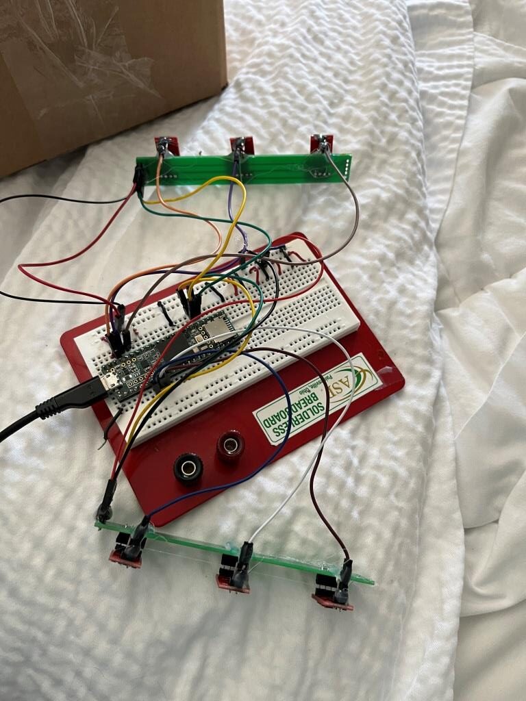
After the usual number of errors, I was able to get a 3-element array of VL53L1X units working with a Teensy 3.5 on a plugboard, and then I moved the sensors to my newly-arrived V2 PCB’s, as shown in the following photo:
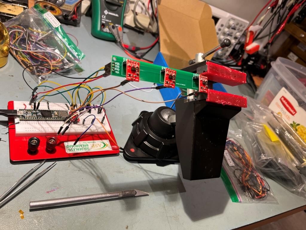
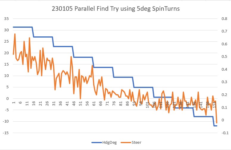
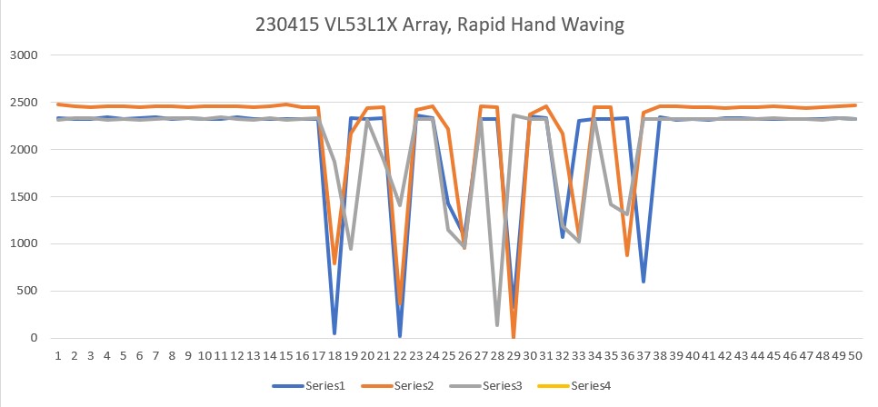
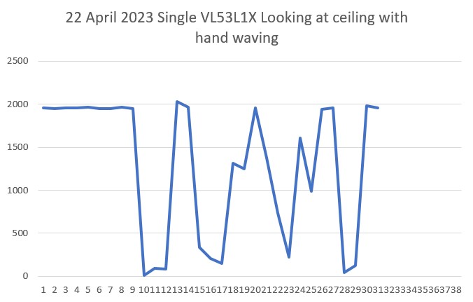
As shown in the photo, the array was pointed diagonally up toward the ceiling about 2.4-2.5m away, while the test was running, I waved my hand rapidly back and forth through the ‘beam’, to see how quickly the sensors could react. As shown in the following Excel plot, the answer is “pretty darned quickly!”.
My wife and I spent last week in Gatlinburg, Tenn. For those of you who have never heard of Gatlinburg, it is a small town nestled in the Great Smoky Mountains National Park. For most people, it is known for it’s beautiful scenery, great shopping, and its colorful history. However, for us bridge buffs, it is famous as the host of a regional bridge tournament, one of the largest in the nation.
There is a fair amount of down time between games, so I brought my VL53L1X test setup along to play with. This morning I was able to test my two new 3-element VL53L1X arrays connected to a Teensy 3.5 on a plugboard as shown in the following photo:
I used my ‘VL53L1X_Pololu_V1.ino’ (shown in it’s entirety below) to test the arrays.
|
1 2 3 4 5 6 7 8 9 10 11 12 13 14 15 16 17 18 19 20 21 22 23 24 25 26 27 28 29 30 31 32 33 34 35 36 37 38 39 40 41 42 43 44 45 46 47 48 49 50 51 52 53 54 55 56 57 58 59 60 61 62 63 64 65 66 67 68 69 70 71 72 73 74 75 76 77 78 79 80 81 82 83 84 85 86 87 88 89 90 91 92 93 94 95 96 97 98 99 100 101 102 103 104 105 106 |
/* Name: VL53L1X_Pololu_V1.ino Created: 4/14/2023 4:55:00 PM Author: FRANKNEWXPS15\Frank */ /* This example shows how to set up and read multiple VL53L1X sensors connected to the same I2C bus. Each sensor needs to have its XSHUT pin connected to a different Arduino pin, and you should change sensorCount and the xshutPins array below to match your setup. For more information, see ST's application note AN4846 ("Using multiple VL53L0X in a single design"). The principles described there apply to the VL53L1X as well. */ #include <Wire.h> #include <VL53L1X.h> // The number of sensors in your system. const uint8_t sensorCount = 5; //const uint8_t sensorCount = 6; // The Arduino pin connected to the XSHUT pin of each sensor. //const uint8_t xshutPins[sensorCount] = { 4, 5, 6 }; //const uint8_t xshutPins[sensorCount] = {32,31,30};//04/14/23 //const uint8_t xshutPins[sensorCount] = {23,22,21};//04/14/23 //const uint8_t xshutPins[sensorCount] = {5,6,7};//04/14/23 //const uint8_t xshutPins[sensorCount] = {23,22,21,5,6,7};//04/14/23 const uint8_t xshutPins[sensorCount] = {23,22,21,7,6};//04/14/23 VL53L1X sensors[sensorCount]; void setup() { while (!Serial) {} Serial.begin(115200); delay(2000); //04/14/23 needed for Teensy Wire.begin(); Wire1.begin(); Wire2.begin(); //Wire.setClock(400000); // use 400 kHz I2C //move sensors to Wire1 for (uint8_t i = 0; i < sensorCount; i++) { //sensors[i].setBus(&Wire2); sensors[i].setBus(&Wire1); } // Disable/reset all sensors by driving their XSHUT pins low. for (uint8_t i = 0; i < sensorCount; i++) { pinMode(xshutPins[i], OUTPUT); digitalWrite(xshutPins[i], LOW); Serial.printf("Set pin %d LOW\n", xshutPins[i]); } // Enable, initialize, and start each sensor, one by one. for (uint8_t i = 0; i < sensorCount; i++) { // Stop driving this sensor's XSHUT low. This should allow the carrier // board to pull it high. (We do NOT want to drive XSHUT high since it is // not level shifted.) Then wait a bit for the sensor to start up. //pinMode(xshutPins[i], INPUT); digitalWrite(xshutPins[i], HIGH); Serial.printf("Set pin %d to HIGH\n", xshutPins[i]); delay(10); //delay(100); sensors[i].setTimeout(500); if (!sensors[i].init()) { Serial.print("Failed to detect and initialize sensor "); Serial.println(i); while (1); } else { Serial.printf("init() succeeded for sensor %d\n", i); } // Each sensor must have its address changed to a unique value other than // the default of 0x29 (except for the last one, which could be left at // the default). To make it simple, we'll just count up from 0x2A. sensors[i].setAddress(0x2A + i); //sensors[i].setAddress(0x3A + i); Serial.printf("sensor %d I2C address set to 0X%X\n",i, sensors[i].getAddress()); sensors[i].startContinuous(50); } } void loop() { for (uint8_t i = 0; i < sensorCount; i++) { Serial.print(sensors[i].read()); if (sensors[i].timeoutOccurred()) { Serial.print(" TIMEOUT"); } Serial.print('\t'); } Serial.println(); } |
This program instantiates an array of VL53L1X objects named ‘sensors’, and the user initializes this array with the pin numbers attached to the XSHUT input of each device. In its original ‘out of the box’ configuration, the program expects three sensors to be attached to the default I2C port (Wire0), with XSHUT lines connected to controller pins 4, 5, & 6. As I described earlier in my 15 April update, I first modified the program to use Teensy 3.5 pins 32, 31, & 30 and verified that all three sensors were recognized and produced good data. Then I added a second 3-element sensor array on the same I2C bus, with XSHUT pins tied to Teensy 3.5 pins 4,5, & 6. Unfortunately, the program refused to recognize any of the sensors on the second array. So, I used the ‘sensorCount’ value and the contents of the xshutPins[sensorCount] array to selectively disable individual sensors on the second array, and I was able to determine that one of the VL53L1X sensors on the second array wasn’t responding for some reason, but the other two worked find. So, now I know that the Wire1 I2C bus on the Teensy 3.5 can handle at least 5 sensors, with no external pullup resistors – yay!
The next step was to move one of the arrays to Wire2 to more closely emulate the current situation on the robot. Here is the completed code, with only two of the three elements in the second array being utilized:
|
1 2 3 4 5 6 7 8 9 10 11 12 13 14 15 16 17 18 19 20 21 22 23 24 25 26 27 28 29 30 31 32 33 34 35 36 37 38 39 40 41 42 43 44 45 46 47 48 49 50 51 52 53 54 55 56 57 58 59 60 61 62 63 64 65 66 67 68 69 70 71 72 73 74 75 76 77 78 79 80 81 82 83 84 85 86 87 88 89 90 91 92 93 94 95 96 97 98 99 100 101 102 103 104 105 106 107 108 109 110 111 112 113 114 115 116 117 118 119 120 121 122 123 124 125 126 127 128 129 130 131 132 133 134 135 136 137 138 139 140 141 142 143 144 145 146 147 148 149 150 151 152 153 154 155 156 157 158 159 |
/* Name: VL53L1X_Pololu_V1.ino Created: 4/14/2023 4:55:00 PM Author: FRANKNEWXPS15\Frank */ /* This example shows how to set up and read multiple VL53L1X sensors connected to the same I2C bus. Each sensor needs to have its XSHUT pin connected to a different Arduino pin, and you should change sensorCount and the xshutPins array below to match your setup. For more information, see ST's application note AN4846 ("Using multiple VL53L0X in a single design"). The principles described there apply to the VL53L1X as well. */ #include <Wire.h> #include <VL53L1X.h> // The number of sensors in your system. //const uint8_t sensorCount = 5; //const uint8_t sensorCount = 6; const uint8_t Wire1sensorCount = 3; const uint8_t Wire2sensorCount = 2; // The Arduino pin connected to the XSHUT pin of each sensor. //const uint8_t xshutPins[sensorCount] = { 4, 5, 6 }; //const uint8_t xshutPins[sensorCount] = {32,31,30};//04/14/23 //const uint8_t xshutPins[sensorCount] = {23,22,21};//04/14/23 //const uint8_t xshutPins[sensorCount] = {5,6,7};//04/14/23 //const uint8_t xshutPins[sensorCount] = {23,22,21,5,6,7};//04/14/23 const uint8_t Wire1xshutPins[Wire1sensorCount] = {23,22,21};//04/14/23 const uint8_t Wire2xshutPins[Wire2sensorCount] = {6,7};//04/14/23 VL53L1X Wire1sensors[Wire1sensorCount]; VL53L1X Wire2sensors[Wire2sensorCount]; void setup() { while (!Serial) {} Serial.begin(115200); delay(2000); //04/14/23 needed for Teensy Wire.begin(); Wire1.begin(); Wire2.begin(); //move some sensors to Wire1 for (uint8_t i = 0; i < Wire1sensorCount; i++) { //sensors[i].setBus(&Wire2); Wire1sensors[i].setBus(&Wire1); } for (uint8_t i = 0; i < Wire2sensorCount; i++) { //sensors[i].setBus(&Wire2); Wire2sensors[i].setBus(&Wire2); } // Disable/reset all sensors by driving their XSHUT pins low. for (uint8_t i = 0; i < Wire1sensorCount; i++) { pinMode(Wire1xshutPins[i], OUTPUT); digitalWrite(Wire1xshutPins[i], LOW); Serial.printf("Set pin %d LOW\n", Wire1xshutPins[i]); } for (uint8_t i = 0; i < Wire2sensorCount; i++) { pinMode(Wire2xshutPins[i], OUTPUT); digitalWrite(Wire2xshutPins[i], LOW); Serial.printf("Set pin %d LOW\n", Wire2xshutPins[i]); } // Enable, initialize, and start each sensor, one by one. for (uint8_t i = 0; i < Wire1sensorCount; i++) { // Stop driving this sensor's XSHUT low. This should allow the carrier // board to pull it high. (We do NOT want to drive XSHUT high since it is // not level shifted.) Then wait a bit for the sensor to start up. //pinMode(xshutPins[i], INPUT); digitalWrite(Wire1xshutPins[i], HIGH); Serial.printf("Set pin %d to HIGH\n", Wire1xshutPins[i]); delay(10); //delay(100); Wire1sensors[i].setTimeout(500); if (!Wire1sensors[i].init()) { Serial.print("Failed to detect and initialize sensor "); Serial.println(i); while (1); } else { Serial.printf("init() succeeded for sensor %d\n", i); } // Each sensor must have its address changed to a unique value other than // the default of 0x29 (except for the last one, which could be left at // the default). To make it simple, we'll just count up from 0x2A. Wire1sensors[i].setAddress(0x2A + i); //sensors[i].setAddress(0x3A + i); Serial.printf("sensor %d I2C address set to 0X%X\n",i, Wire1sensors[i].getAddress()); Wire1sensors[i].startContinuous(50); } for (uint8_t i = 0; i < Wire2sensorCount; i++) { // Stop driving this sensor's XSHUT low. This should allow the carrier // board to pull it high. (We do NOT want to drive XSHUT high since it is // not level shifted.) Then wait a bit for the sensor to start up. //pinMode(xshutPins[i], INPUT); digitalWrite(Wire2xshutPins[i], HIGH); Serial.printf("Set pin %d to HIGH\n", Wire2xshutPins[i]); delay(10); //delay(100); Wire2sensors[i].setTimeout(500); if (!Wire2sensors[i].init()) { Serial.print("Failed to detect and initialize sensor "); Serial.println(i); while (1); } else { Serial.printf("init() succeeded for sensor %d\n", i); } // Each sensor must have its address changed to a unique value other than // the default of 0x29 (except for the last one, which could be left at // the default). To make it simple, we'll just count up from 0x2A. Wire2sensors[i].setAddress(0x2A + i); //sensors[i].setAddress(0x3A + i); Serial.printf("sensor %d I2C address set to 0X%X\n", i, Wire2sensors[i].getAddress()); Wire2sensors[i].startContinuous(50); } } void loop() { for (uint8_t i = 0; i < Wire1sensorCount; i++) { Serial.print(Wire1sensors[i].read()); if (Wire1sensors[i].timeoutOccurred()) { Serial.print(" TIMEOUT"); } Serial.print('\t'); } for (uint8_t i = 0; i < Wire2sensorCount; i++) { Serial.print(Wire2sensors[i].read()); if (Wire2sensors[i].timeoutOccurred()) { Serial.print(" TIMEOUT"); } Serial.print('\t'); } Serial.println(); } |
Here is a short section of the output from the above program:
|
1 2 3 4 5 6 7 8 9 10 11 12 13 14 15 16 17 18 19 20 21 22 23 24 25 26 27 28 29 30 31 32 33 34 35 36 37 38 39 40 41 42 43 44 45 46 47 48 49 50 51 52 53 54 55 56 57 58 59 60 61 62 63 64 65 66 67 68 69 70 71 72 73 74 75 76 77 78 79 80 81 82 83 84 85 |
Opening port Port open Set pin 23 LOW Set pin 22 LOW Set pin 21 LOW Set pin 6 LOW Set pin 7 LOW Set pin 23 to HIGH got 0XEACC from readReg16Bit(IDENTIFICATION__MODEL_ID) Inside setDistanceMode(DistanceMode 2) init() succeeded for sensor 0 sensor 0 I2C address set to 0X2A Set pin 22 to HIGH got 0XEACC from readReg16Bit(IDENTIFICATION__MODEL_ID) Inside setDistanceMode(DistanceMode 2) init() succeeded for sensor 1 sensor 1 I2C address set to 0X2B Set pin 21 to HIGH got 0XEACC from readReg16Bit(IDENTIFICATION__MODEL_ID) Inside setDistanceMode(DistanceMode 2) init() succeeded for sensor 2 sensor 2 I2C address set to 0X2C Set pin 6 to HIGH got 0XEACC from readReg16Bit(IDENTIFICATION__MODEL_ID) Inside setDistanceMode(DistanceMode 2) init() succeeded for sensor 0 sensor 0 I2C address set to 0X2A Set pin 7 to HIGH got 0XEACC from readReg16Bit(IDENTIFICATION__MODEL_ID) Inside setDistanceMode(DistanceMode 2) init() succeeded for sensor 1 sensor 1 I2C address set to 0X2B 3471 2932 180 462 389 3479 2950 170 473 397 3423 2942 196 471 396 3434 2926 178 471 397 3529 2931 183 473 398 3457 2932 176 472 396 3466 2951 188 472 400 3483 2938 191 470 397 3431 2920 175 470 400 3473 2946 169 474 395 3496 2932 198 471 394 3496 2920 173 474 399 3422 2962 180 473 400 3450 2962 183 472 393 3468 2929 174 476 401 3429 2936 181 472 395 3483 2956 171 473 397 3496 2914 195 471 392 3447 2948 193 473 401 3474 2958 170 475 392 3506 2945 164 473 397 3530 2959 164 471 393 3461 2944 175 471 399 3521 2957 163 474 395 3516 2939 160 473 394 3490 2940 176 472 396 3472 2940 169 471 396 3445 2948 168 476 397 3490 2968 174 473 395 3489 2929 166 474 393 3411 2933 186 473 396 3501 2948 179 471 398 3526 2932 182 473 396 3521 2945 185 471 392 3476 2946 191 473 396 3502 2958 172 473 396 3484 2937 174 472 396 3521 2942 182 474 398 3438 2944 175 473 397 3515 2941 202 472 399 3488 2960 190 472 397 3471 2951 186 474 398 3524 2941 191 473 395 3504 2979 174 472 392 3501 2918 177 472 396 3463 2941 184 472 397 3440 2943 185 471 392 3495 2940 175 474 397 3492 2910 183 475 395 3460 2946 174 470 398 3454 2939 203 476 394 3451 2955 Port closed |
From the above telemetry I have picked out the following lines:
|
1 2 3 4 5 6 |
sensor 0 I2C address set to 0X2A sensor 1 I2C address set to 0X2B sensor 2 I2C address set to 0X2C sensor 0 I2C address set to 0X2A sensor 1 I2C address set to 0X2B |
Note that in the above there are two sensors set for 0X2A and two for 0X2B. This works, because the first three sensors (0, 1, & 2) are on the Wire1 I2C bus, and the remaining two (also sensors 0 & 1) are on the Wire2 bus. This setup essentially duplicates the dual 3-element sensor arrays on WallE3.
After getting the above program working with Wire1 & Wire2, I used it to modify my previous Teensy_VL53L0X_I2C_Slave_V4.ino program to use the new VL53L1X sensors. The new program , ‘Teensy_VL53L1X_I2C_Slave_V4.ino’ is shown in it’s entirety below:
|
1 2 3 4 5 6 7 8 9 10 11 12 13 14 15 16 17 18 19 20 21 22 23 24 25 26 27 28 29 30 31 32 33 34 35 36 37 38 39 40 41 42 43 44 45 46 47 48 49 50 51 52 53 54 55 56 57 58 59 60 61 62 63 64 65 66 67 68 69 70 71 72 73 74 75 76 77 78 79 80 81 82 83 84 85 86 87 88 89 90 91 92 93 94 95 96 97 98 99 100 101 102 103 104 105 106 107 108 109 110 111 112 113 114 115 116 117 118 119 120 121 122 123 124 125 126 127 128 129 130 131 132 133 134 135 136 137 138 139 140 141 142 143 144 145 146 147 148 149 150 151 152 153 154 155 156 157 158 159 160 161 162 163 164 165 166 167 168 169 170 171 172 173 174 175 176 177 178 179 180 181 182 183 184 185 186 187 188 189 190 191 192 193 194 195 196 197 198 199 200 201 202 203 204 205 206 207 208 209 210 211 212 213 214 215 216 217 218 219 220 221 222 223 224 225 226 227 228 229 230 231 232 233 234 235 236 237 238 239 240 241 242 243 244 245 246 247 248 249 250 251 252 253 254 255 256 257 258 259 260 261 262 263 264 265 266 267 268 269 270 271 272 273 274 275 276 277 278 279 280 281 282 283 284 285 286 287 288 289 290 291 292 293 294 295 296 297 298 299 300 301 302 303 304 305 306 307 308 309 310 311 312 313 314 315 316 317 318 319 320 321 322 323 324 325 326 327 328 329 330 331 332 333 334 335 336 337 338 339 340 341 342 343 344 345 346 347 348 349 350 351 352 353 354 355 356 357 358 359 360 361 362 363 364 365 366 367 368 369 370 371 372 373 374 375 376 377 378 379 380 381 382 383 384 385 386 387 388 389 390 391 392 393 394 395 396 397 398 399 400 401 402 403 404 405 406 407 408 409 410 411 412 413 414 415 416 417 418 419 420 421 422 423 424 425 426 427 428 429 430 431 432 433 434 435 436 437 438 439 440 441 442 443 444 445 446 447 448 449 450 451 452 453 454 455 456 457 458 459 460 461 462 463 464 465 466 467 468 469 470 471 472 473 474 475 476 477 478 479 480 481 482 483 484 485 486 487 488 489 490 491 492 493 494 495 496 497 498 499 500 501 502 503 504 505 506 507 508 509 510 511 512 513 514 515 516 517 518 519 520 521 522 523 524 525 526 527 528 529 530 531 532 533 534 535 536 537 538 539 540 541 542 543 544 545 546 547 548 549 550 551 552 553 554 555 556 557 558 559 560 561 562 563 564 565 566 567 568 569 570 571 572 573 574 575 576 577 578 579 580 581 582 583 584 585 586 587 588 589 590 591 592 593 594 595 596 597 598 599 600 601 602 603 604 605 606 607 608 609 610 611 612 613 614 615 616 617 618 619 620 621 622 623 624 625 626 627 628 629 630 631 632 633 634 635 636 637 638 639 640 641 642 643 644 645 646 647 648 649 650 651 652 653 654 655 656 657 658 659 660 661 662 663 664 665 666 667 668 669 670 671 672 673 674 675 676 677 678 679 680 681 682 683 684 685 686 687 688 689 690 691 692 693 694 |
/* Name: Teensy_7VL53L1X_I2C_Slave_V1.ino Created: 4/12/2023 3:40:21 PM Author: FRANKNEWXPS15\Frank Notes: 04/12/23 Copied from Teensy_7VL53L10X_I2C_Slave_V4 and revised to use VL53L1X sensors instead of VL53L0X, and the Pololu VL53L1X library instead of the VL53L0X one 04/21/23 code ported from VL53L1X_Pololu_V1.ino */ #pragma region EARLIER_VERSIONS /* Name: Teensy_7VL53L1X_I2C_Slave_V4.ino Created: 4/3/2022 1:04:28 PM Author: FRANKNEWXPS15\Frank Notes: 04/03/22 This version adds a linear distance correction algorithm to each VL53L1X 11/17/22 changed measurement budget from 20 to 50mSec for right-side sensors only 11/20/22 changed measurement budget from 20 to 50mSec for left-side and rear sensors 12/14/22 changed measurement budget back to 30mSec from 50mSec for all sensors */ /* Name: Teensy_7VL53L1X_I2C_Slave_V3.ino Created: 1/24/2021 4:03:35 PM Author: FRANKNEWXPS15\Frank This is the 'final' version of the Teensy 3.5 project to manage all seven VL53L1X lidar distance sensors, three on left, three on right, and now including a rear distance sensor. As of this date it was an identical copy of the TeensyHexVL53L1XHighSpeedDemo project, just renamed for clarity 01/23/22 - revised to work properly with Teensy 3.5 main processor */ /* Name: TeensyHexVL53L1XHighSpeedDemo.ino Created: 10/1/2020 3:49:01 PM Author: FRANKNEWXPS15\Frank This demo program combines the code from my Teensy_VL53L1X_I2C_Slave_V2 project with the VL53L1X 'high speed' code from the Pololu support forum post at https://forum.pololu.com/t/high-speed-with-vl53l0x/16585/3 */ /* Name: Teensy_VL53L1X_I2C_Slave_V2.ino Created: 8/4/2020 7:42:22 PM Author: FRANKNEWXPS15\Frank This project merges KurtE's multi-wire capable version of Pololu's VL53L1X library with my previous Teensy_VL53L1X_I2C_Slave project, which used the Adafruit VL53L1X library. This (hopefully) will be the version uploaded to the Teensy on the 2nd deck of Wall-E2 and which controls the left & right 3-VL53L1X sensor arrays 01/17/22: Copied VL53L1X.h/cpp from C:\Users\paynt\Documents\Arduino\Libraries\vl53l0x-arduino-multi_wire so I won't have to guess which library folder these files came from 01/17/22: if you have a local file.h same as a library\xx\file.h, then if VMicro's 'deep search'option is enabled, must use #include "file.h" instead of #include <file.h>. This is the reason for using #include "VL53L1X.h" and #include "I2C_Anything.h" below 01/17/22 the local version of "I2C_Anything.h" uses '#include <i2c_t3.h>' vice <Wire.h> for multiple I2C buss availability. 01/18/22 removed I2C_Anything.h & VL53L1X.h from project folder so can use library versions 01/22/22 added #ifdef NO_VL53L1X and assoc #ifndef blocks for debug */ #pragma endregion EARLIER_VERSIONS #include <Wire.h> //01/18/22 Wire.h has multiple I2C bus access capability #include <VL53L1X.h> #include <I2C_Anything.h> #include "elapsedMillis.h" #pragma region DEFINES //#define NO_VL53L1X #define __FILENAME__ (strrchr(__FILE__, '\\') ? strrchr(__FILE__, '\\') + 1 : __FILE__) //added 01/26/23 to extract pgm filename from full path #pragma endregion DEFINES enum VL53L1X_REQUEST { VL53L1X_READYCHECK, //added 11/10/20 to prevent bad reads during Teensy setup() VL53L1X_CENTERS_ONLY, VL53L1X_RIGHT, VL53L1X_LEFT, VL53L1X_ALL, //added 08/05/20, chg 'BOTH' to 'ALL' 10/31/20 VL53L1X_REAR_ONLY //added 10/24/20 }; #pragma region GLOBALS volatile uint8_t request_type; const int SETUP_DURATION_OUTPUT_PIN = 33; const int REQUEST_EVENT_DURATION_OUTPUT_PIN = 34; bool bTeensyReady = false; //const int MSEC_BETWEEN_LED_TOGGLES = 100; const int MSEC_BETWEEN_LED_TOGGLES = 300;//02/21/22 chg so can visually detect live I2C xfrs elapsedMillis mSecBetweenLEDToggle; //right side array uint16_t RF_Dist_mm; uint16_t RC_Dist_mm; uint16_t RR_Dist_mm; //left side array & rear uint16_t LF_Dist_mm; uint16_t LC_Dist_mm; uint16_t LR_Dist_mm; uint16_t Rear_Dist_mm; //02/20/22 back to using float for steer values float RightSteeringVal; float LeftSteeringVal; const int SLAVE_ADDRESS = 0x20; //(32Dec) just a guess for now const int DEFAULT_VL53L1X_ADDR = 0x29; //XSHUT required for I2C address init //right side array const int RF_XSHUT_PIN = 23; const int RC_XSHUT_PIN = 22; const int RR_XSHUT_PIN = 21; //left side array const int LF_XSHUT_PIN = 5; const int LC_XSHUT_PIN = 6; const int LR_XSHUT_PIN = 7; const int Rear_XSHUT_PIN = 8; //const int MAX_LIDAR_RANGE_MM = 1000; //make it obvious when nearest object is out of range const int MAX_LIDAR_RANGE_MM = 3000; //VL53L1X can go out past 3m //04/15/23 The Pololu VL53L1X library uses a parameterless constructor // and a subsequent 'setBus()' function to change the I2C bus //right side array VL53L1X lidar_RF; VL53L1X lidar_RC; VL53L1X lidar_RR; //left side array VL53L1X lidar_LF; VL53L1X lidar_LC; VL53L1X lidar_LR; VL53L1X lidar_Rear; #pragma endregion GLOBALS void setup() { bTeensyReady = false; //11/10/20 prevent bad data reads by main controller Serial.begin(115200); // wait until serial port opens delay(3000); Wire.begin(SLAVE_ADDRESS); //set Teensy Wire0 port up as slave Wire.onRequest(requestEvent); //ISR for I2C requests from master (Mega 2560) Wire.onReceive(receiveEvent); //ISR for I2C data from master (Mega 2560) //initialize Wire1 & Wire2 to talk to the two arrays, plus the rear sensor Wire1.begin(); Wire2.begin(); Serial.printf("Teensy_7VL53L1X_I2C_Slave_V1\n\n"); #pragma region PIN_INITIALIZATION pinMode(SETUP_DURATION_OUTPUT_PIN, OUTPUT); pinMode(REQUEST_EVENT_DURATION_OUTPUT_PIN, OUTPUT); pinMode(LED_BUILTIN, OUTPUT); digitalWrite(SETUP_DURATION_OUTPUT_PIN, HIGH); //right-side XSHUT control pins pinMode(RF_XSHUT_PIN, OUTPUT); pinMode(RC_XSHUT_PIN, OUTPUT); pinMode(RR_XSHUT_PIN, OUTPUT); //left-side XSHUT control pins pinMode(LF_XSHUT_PIN, OUTPUT); pinMode(LC_XSHUT_PIN, OUTPUT); pinMode(LR_XSHUT_PIN, OUTPUT); pinMode(Rear_XSHUT_PIN, OUTPUT); #pragma endregion PIN_INITIALIZATION #pragma region VL53L1X_INIT //04/15/23 The Pololu VL53L1X library uses a parameterless constructor // and a subsequent 'setBus()' function to change the I2C bus //left side array I2C SLC2/SDA2 pins 3/4 lidar_LF.setBus(&Wire2); lidar_LC.setBus(&Wire2); lidar_LR.setBus(&Wire2); //right side array I2C SLC0/SDA0 pins 27/28 lidar_RF.setBus(&Wire1); lidar_RC.setBus(&Wire1); lidar_RR.setBus(&Wire1); //Put all sensors in reset mode by pulling XSHUT low digitalWrite(RF_XSHUT_PIN, LOW); digitalWrite(RC_XSHUT_PIN, LOW); digitalWrite(RR_XSHUT_PIN, LOW); digitalWrite(LF_XSHUT_PIN, LOW); digitalWrite(LC_XSHUT_PIN, LOW); digitalWrite(LR_XSHUT_PIN, LOW); digitalWrite(Rear_XSHUT_PIN, LOW); //now bring lidar_RF only out of reset and set it's address //input w/o pullups sets line to high impedance so XSHUT pullup to 3.3V takes over pinMode(RF_XSHUT_PIN, INPUT); delay(10); if (!lidar_RF.init()) { Serial.println("Failed to detect and initialize lidar_RF!"); while (1) {} } //from Pololu forum post lidar_RF.setMeasurementTimingBudget(30000); //11/20/22 //lidar_RF.setMeasurementTimingBudget(50000); //11/17/22 lidar_RF.startContinuous(50); lidar_RF.setAddress(DEFAULT_VL53L1X_ADDR + 1); Serial.printf("lidar_RF address is 0x%x\n", lidar_RF.getAddress()); //now bring lidar_RC only out of reset, initialize it, and set its address //input w/o pullups sets line to high impedance so XSHUT pullup to 3.3V takes over pinMode(RC_XSHUT_PIN, INPUT); delay(10); if (!lidar_RC.init()) { Serial.println("Failed to detect and initialize lidar_RC!"); while (1) {} } //from Pololu forum post lidar_RC.setMeasurementTimingBudget(30000); //11/20/22 //lidar_RC.setMeasurementTimingBudget(50000); //11/17/22 lidar_RC.startContinuous(50); lidar_RC.setAddress(DEFAULT_VL53L1X_ADDR + 2); Serial.printf("lidar_RC address is 0x%x\n", lidar_RC.getAddress()); //now bring lidar_RR only out of reset, initialize it, and set its address //input w/o pullups sets line to high impedance so XSHUT pullup to 3.3V takes over pinMode(RR_XSHUT_PIN, INPUT); delay(10); if (!lidar_RR.init()) { Serial.println("Failed to detect and initialize lidar_RR!"); while (1) {} } //from Pololu forum post lidar_RR.setMeasurementTimingBudget(30000); //11/20/22 //lidar_RR.setMeasurementTimingBudget(50000); //11/17/22 lidar_RR.startContinuous(50); lidar_RR.setAddress(DEFAULT_VL53L1X_ADDR + 3); Serial.printf("lidar_RR address is 0x%x\n", lidar_RR.getAddress()); //now bring lidar_LF only out of reset, initialize it, and set its address //input w/o pullups sets line to high impedance so XSHUT pullup to 3.3V takes over pinMode(LF_XSHUT_PIN, INPUT); delay(10); if (!lidar_LF.init()) { Serial.println("Failed to detect and initialize lidar_LF!"); while (1) {} } //from Pololu forum post lidar_LF.setMeasurementTimingBudget(30000); //lidar_LF.setMeasurementTimingBudget(50000); //11/20/22 lidar_LF.startContinuous(50); lidar_LF.setAddress(DEFAULT_VL53L1X_ADDR + 4); Serial.printf("lidar_LF address is 0x%x\n", lidar_LF.getAddress()); //now bring lidar_LC only out of reset, initialize it, and set its address //input w/o pullups sets line to high impedance so XSHUT pullup to 3.3V takes over pinMode(LC_XSHUT_PIN, INPUT); delay(10); if (!lidar_LC.init()) { Serial.println("Failed to detect and initialize lidar_LC!"); while (1) {} } //from Pololu forum post lidar_LC.setMeasurementTimingBudget(30000); //lidar_LC.setMeasurementTimingBudget(50000); //11/20/22 lidar_LC.startContinuous(50); lidar_LC.setAddress(DEFAULT_VL53L1X_ADDR + 5); Serial.printf("lidar_LC address is 0x%x\n", lidar_LC.getAddress()); //now bring lidar_LR only out of reset, initialize it, and set its address //input w/o pullups sets line to high impedance so XSHUT pullup to 3.3V takes over pinMode(LR_XSHUT_PIN, INPUT); if (!lidar_LR.init()) { Serial.println("Failed to detect and initialize lidar_LR!"); while (1) {} } //from Pololu forum post lidar_LR.setMeasurementTimingBudget(30000); //lidar_LR.setMeasurementTimingBudget(50000); //11/20/22 lidar_LR.startContinuous(50); lidar_LR.setAddress(DEFAULT_VL53L1X_ADDR + 6); Serial.printf("lidar_LR address is 0x%x\n", lidar_LR.getAddress()); //added 10/23/20 for rear sensor //now bring lidar_Rear only out of reset, initialize it, and set its address //input w/o pullups sets line to high impedance so XSHUT pullup to 3.3V takes over pinMode(Rear_XSHUT_PIN, INPUT); if (!lidar_Rear.init()) { Serial.println("Failed to detect and initialize lidar_Rear!"); while (1) {} } //from Pololu forum post lidar_Rear.setMeasurementTimingBudget(30000); //lidar_Rear.setMeasurementTimingBudget(50000); //11/20/22 lidar_Rear.startContinuous(50); lidar_Rear.setAddress(DEFAULT_VL53L1X_ADDR + 7); Serial.printf("lidar_Rear address is 0x%x\n", lidar_Rear.getAddress()); #pragma endregion VL53L1X_INIT digitalWrite(SETUP_DURATION_OUTPUT_PIN, LOW); bTeensyReady = true; //11/10/20 added to prevent bad data reads by main controller mSecBetweenLEDToggle = 0; Serial.printf("Msec\tLFront\tLCtr\tLRear\tRFront\tRCtr\tRRear\tRear\tLSteer\tRSteer\n"); } void loop() { } void requestEvent() { //Purpose: Send requested sensor data to the Mega controller via main I2C bus //Inputs: // request_type = uint8_t value denoting type of data requested (from receiveEvent()) // 0 = left & right center distances only // 1 = right side front, center and rear distances, plus steering value // 2 = left side front, center and rear distances, plus steering value // 3 = both side front, center and rear distances, plus both steering values //Outputs: // Requested data sent to master //Notes: // 08/05/20 added VL53L1X_ALL request type to get both sides at once // 10/24/20 added VL53L1X_REAR_ONLY request type // 11/09/20 added write to pin for O'scope monitoring //DEBUG!! //int data_size = 0; //DEBUG!! //DEBUG!! //Serial.printf("RequestEvent() with request_type = %d: VL53L0X Front/Center/Rear distances = %d, %d, %d\n", // request_type, RF_Dist_mm, RC_Dist_mm, RR_Dist_mm); //DEBUG!! //digitalWrite(LED_BUILTIN, HIGH);//added 01/22/22 digitalWrite(REQUEST_EVENT_DURATION_OUTPUT_PIN, HIGH); digitalToggle(LED_BUILTIN);//2/21/22 added for visual indication of I2C activity switch (request_type) { case VL53L1X_READYCHECK: //added 11/10/20 to prevent bad reads during Teensy setup() Serial.printf("in VL53L1X_READYCHECK case at %lu with bTeensyReady = %d\n", millis(), bTeensyReady); I2C_writeAnything(bTeensyReady); break; case VL53L1X_CENTERS_ONLY: //DEBUG!! //data_size = 2*sizeof(uint16_t); //Serial.printf("Sending %d bytes LC_Dist_mm = %d, RC_Dist_mm = %d to master\n", data_size, LC_Dist_mm, RC_Dist_mm); //DEBUG!! I2C_writeAnything(RC_Dist_mm); I2C_writeAnything(LC_Dist_mm); break; case VL53L1X_RIGHT: //DEBUG!! //data_size = 3 * sizeof(uint16_t) + sizeof(float); //Serial.printf("Sending %d bytes RF/RC/RR/RS vals = %d, %d, %d, %3.2f to master\n", // data_size, RF_Dist_mm, RC_Dist_mm, RR_Dist_mm, RightSteeringVal); //DEBUG!! I2C_writeAnything(RF_Dist_mm); I2C_writeAnything(RC_Dist_mm); I2C_writeAnything(RR_Dist_mm); I2C_writeAnything(RightSteeringVal); break; case VL53L1X_LEFT: //DEBUG!! //data_size = 3 * sizeof(uint16_t) + sizeof(float); //Serial.printf("Sending %d bytes LF/LC/LR/LS vals = %d, %d, %d, %3.2f to master\n", // data_size, LF_Dist_mm, LC_Dist_mm, LR_Dist_mm, LeftSteeringVal); //DEBUG!! I2C_writeAnything(LF_Dist_mm); I2C_writeAnything(LC_Dist_mm); I2C_writeAnything(LR_Dist_mm); I2C_writeAnything(LeftSteeringVal); break; case VL53L1X_ALL: //Serial.printf("In VL53L1X_ALL case\n"); //added 08/05/20 to get data from both sides at once //10/31/20 chg to VL53L1X_ALL & report all 7 sensor values //DEBUG!! //data_size = 3 * sizeof(uint16_t) + sizeof(float); //data_size = 7 * sizeof(uint16_t) + 2 * sizeof(float); //Serial.printf("Sending %d bytes to master\n", data_size); //Serial.printf("%d bytes: %d\t%d\t%d\t%3.2f\t%d\t%d\t%d\t%d\t%3.2f\n", // data_size, LF_Dist_mm, LC_Dist_mm, LR_Dist_mm, LeftSteeringVal, // RF_Dist_mm, RC_Dist_mm, RR_Dist_mm, Rear_Dist_mm, RightSteeringVal); //DEBUG!! //DEBUG!! //data_size = 3 * sizeof(uint16_t) + sizeof(float); //Serial.printf("Sending %d bytes LF/LC/LR/LS vals = %d, %d, %d, %3.2f to master\n", // data_size, LF_Dist_mm, LC_Dist_mm, LR_Dist_mm, LeftSteeringVal); //DEBUG!! //left side I2C_writeAnything(LF_Dist_mm); I2C_writeAnything(LC_Dist_mm); I2C_writeAnything(LR_Dist_mm); I2C_writeAnything(LeftSteeringVal); //DEBUG!! //data_size = 3 * sizeof(uint16_t) + sizeof(float); //data_size = 4 * sizeof(uint16_t) + sizeof(float); //Serial.printf("Sending %d bytes RF/RC/RR/R/RS vals = %d, %d, %d, %d, %3.2f to master\n", // data_size, RF_Dist_mm, RC_Dist_mm, RR_Dist_mm, Rear_Dist_mm, RightSteeringVal); //DEBUG!! //right side I2C_writeAnything(RF_Dist_mm); I2C_writeAnything(RC_Dist_mm); I2C_writeAnything(RR_Dist_mm); I2C_writeAnything(Rear_Dist_mm); I2C_writeAnything(RightSteeringVal); break; case VL53L1X_REAR_ONLY: //DEBUG!! //data_size = sizeof(uint16_t); //Serial.printf("Sending %d bytes Rear_Dist_mm = %d to master\n", data_size, Rear_Dist_mm); //DEBUG!! I2C_writeAnything(Rear_Dist_mm); break; default: break; } digitalToggle(LED_BUILTIN);//2/21/22 added for visual indication of I2C activity digitalWrite(REQUEST_EVENT_DURATION_OUTPUT_PIN, LOW); //digitalWrite(LED_BUILTIN, LOW);//added 01/22/22 } void receiveEvent(int numBytes) { //Purpose: capture data request type from Mega I2C master //Inputs: // numBytes = int value denoting number of bytes received from master //Outputs: // uint8_t request_type filled with request type value from master //DEBUG!! //Serial.printf("receiveEvent(%d)\n", numBytes); //DEBUG!! I2C_readAnything(request_type); //DEBUG!! //Serial.printf("receiveEvent: Got %d from master\n", request_type); //DEBUG!! } uint16_t lidar_LF_Correction(uint16_t raw_dist) { //Purpose: Correct for linear error in left front VL53L0X //Provenance: Created 04/03/22 gfp //Inputs: // raw_dist = uint16_t value denoting raw measurement in mm //Outputs: // returns raw_dist (mm) corrected for linear distance measurement error //Notes: // correction = =(raw + 0.4)/1.125 // 04/05/22 bugfix. Raw dist here are MM, but above formula assumed CM - fixed below // correction = =(raw(mm) + 4)/1.125 //uint16_t corrVal = (uint16_t)((float)raw_dist + 0.4f) / 1.125f; //uint16_t corrVal = (uint16_t)((float)raw_dist + 4.f) / 1.125f; //uint16_t corrVal = raw_dist; uint16_t corrVal = (uint16_t)((float)raw_dist - 5.478f) / 1.0918f;//11/20/22 //DEBUG!! //Serial.printf("LF: raw = %d, corr = %d\n", raw_dist, corrVal); //DEBUG!! return corrVal; } uint16_t lidar_LC_Correction(uint16_t raw_dist) { //Purpose: Correct for linear error in left center VL53L0X //Provenance: Created 04/03/22 gfp //Inputs: // raw_dist = uint16_t value denoting raw measurement in mm //Outputs: // returns raw_dist corrected for linear distance measurement error //Notes: // correction = ==(raw - 0.6333)/1.03 // 04/05/22 bugfix. Raw dist here are MM, but above formula assumed CM - fixed below // correction = =(raw(mm) - 6.333)/1.03 //uint16_t corrVal = (uint16_t)((float)raw_dist - 0.6333f) / 1.03f; //uint16_t corrVal = (uint16_t)((float)raw_dist - 6.333f) / 1.03f; //uint16_t corrVal = raw_dist; uint16_t corrVal = (uint16_t)((float)raw_dist - 19.89f) / 0.9913f;//11/20/22 //DEBUG!! //Serial.printf("LC: raw = %d, corr = %d\n", raw_dist, corrVal); //DEBUG!! return corrVal; } uint16_t lidar_LR_Correction(uint16_t raw_dist) { //Purpose: Correct for linear error in left rear VL53L0X //Provenance: Created 04/03/22 gfp //Inputs: // raw_dist = uint16_t value denoting raw measurement in mm //Outputs: // returns raw_dist corrected for linear distance measurement error //Notes: // correction = =raw - 2.0667 // 04/05/22 bugfix. Raw dist here are MM, but above formula assumed CM - fixed below // correction = = raw(mm) - 20.667 //uint16_t corrVal = (uint16_t)((float)raw_dist - 2.0667f); //uint16_t corrVal = (uint16_t)((float)raw_dist - 20.667f); //uint16_t corrVal = raw_dist; uint16_t corrVal = (uint16_t)((float)raw_dist + 9.676f) / 1.1616; //DEBUG!! //Serial.printf("LR: raw = %d, corr = %d\n", raw_dist, corrVal); //DEBUG!! return corrVal; } uint16_t lidar_RF_Correction(uint16_t raw_dist) { //Purpose: Correct for linear error in right front VL53L0X //Provenance: Created 04/03/22 gfp //Inputs: // raw_dist = uint16_t value denoting raw measurement in mm //Outputs: // returns raw_dist corrected for linear distance measurement error in mm //Notes: // correction = =(raw + 0.96)/1.045 // 04/05/22 bugfix. Raw dist here are MM, but above formula assumed CM - fixed below // correction = =(raw(mm) + 9.6f)/1.03f //uint16_t corrVal = (uint16_t)((float)raw_dist + 0.96f) / 1.045f; //uint16_t corrVal = (uint16_t)((float)raw_dist + 9.6f) / 1.045f; //uint16_t corrVal = raw_dist; //11/18/22 uint16_t corrVal = (uint16_t)((float)raw_dist - 4.297f) / 1.0808f; //DEBUG!! //Serial.printf("RF: raw = %d, corr = %d\n", raw_dist, corrVal); //DEBUG!! return corrVal; } uint16_t lidar_RC_Correction(uint16_t raw_dist) { //Purpose: Correct for linear error in right center VL53L0X //Provenance: Created 04/03/22 gfp //Inputs: // raw_dist = uint16_t value denoting raw measurement in mm //Outputs: // returns raw_dist corrected for linear distance measurement error //Notes: // correction = =(raw - 3.2)/1.08 // 04/05/22 bugfix. Raw dist here are MM, but above formula assumed CM - fixed below // correction = =(raw(mm) - 3.2)/1.08 //uint16_t corrVal = (uint16_t)((float)raw_dist - 3.2f) / 1.08f; //uint16_t corrVal = (uint16_t)((float)raw_dist - 32.f) / 1.08f; //uint16_t corrVal = raw_dist; uint16_t corrVal = (uint16_t)((float)raw_dist - 50.603f) / 1.0438f; //DEBUG!! //Serial.printf("RC: raw = %d, corr = %d\n", raw_dist, corrVal); //DEBUG!! return corrVal; } uint16_t lidar_RR_Correction(uint16_t raw_dist) { //Purpose: Correct for linear error in right rear VL53L0X //Provenance: Created 04/03/22 gfp //Inputs: // raw_dist = uint16_t value denoting raw measurement in mm //Outputs: // returns raw_dist corrected for linear distance measurement error //Notes: // correction = =(raw - 3.1)/1.12 // 04/05/22 bugfix. Raw dist here are MM, but above formula assumed CM - fixed below // correction = =(raw(mm) - 31)/1.12 //uint16_t corrVal = (uint16_t)((float)raw_dist - 3.1f) / 1.12f; //uint16_t corrVal = (uint16_t)((float)raw_dist - 31.f) / 1.12f; //uint16_t corrVal = raw_dist; uint16_t corrVal = (uint16_t)((float)raw_dist - 56.746f) / 1.0353; //DEBUG!! //Serial.printf("RR: raw = %d, corr = %d\n", raw_dist, corrVal); //DEBUG!! return corrVal; } uint16_t lidar_Rear_Correction(uint16_t raw_dist) { //Purpose: Correct for linear error in rear VL53L0X //Provenance: Created 04/03/22 gfp //Inputs: // raw_dist = uint16_t value denoting raw measurement in mm //Outputs: // returns raw_dist corrected for linear distance measurement error //Notes: // correction = ==(raw - 1.1)/1.09 // 04/05/22 bugfix. Raw dist here are MM, but above formula assumed CM - fixed below // correction = =(raw(mm) - 11)/1.09 //uint16_t corrVal = (uint16_t)((float)raw_dist - 1.1f) / 1.09f; uint16_t corrVal = (uint16_t)((float)raw_dist - 11.f) / 1.09f; //DEBUG!! //Serial.printf("Rear: raw = %d, corr = %d\n", raw_dist, corrVal); //DEBUG!! return corrVal; } |
22 April 2023 Update:
We got back home from Gatlinburg last night, and so this morning I decided to verify my theory that one of my six VL53L1X distance sensors was indeed defective. I have a pretty healthy skepticism about blaming hardware failures in a hardware/software system; in fact my motto is “Hardware never fails” (it does occasionally fail, but much much less often than a software issue causing the hardware to LOOK like it fails).
So, I loaded my one-sensor VL53L1X_Demo.ino example onto the Teensy 3.5 and used Wire0 (pins 18/19) to drive just this one sensor. Naturally it worked fine, as shwon below:
|
1 2 3 4 5 6 7 8 9 10 11 12 13 14 15 16 17 18 19 20 21 22 23 24 25 26 27 28 29 30 31 32 33 34 35 36 37 38 |
Port open got 0XEACC from readReg16Bit(IDENTIFICATION__MODEL_ID) Inside setDistanceMode(DistanceMode 2) Inside setDistanceMode(DistanceMode 2) 1956 1952 1953 1957 1964 1952 1951 1963 1951 9 94 83 2030 1961 333 208 150 1313 1248 1957 1379 736 220 1607 992 1943 1957 42 121 1985 1956 Port closed |
Well, as I suspected, the hardware seems OK so now I have to figure out why it didn’t respond properly in my six-element setup.
I replaced the ‘XSHUT’ wire from Teensy pin 5 to the sensor, but this did not solve the problem. I also tried driving the XSHUT line HIGH instead of letting it float, but no joy. Next I tried switching the suspect sensor with the one right next to it, to see if the problem follows the sensor. After several iterations, it now appears that the problem stays with the sensor associated with whatever sensor’s XSHUT pin is connected to Teensy 3.5 pin 5, or possibly with the 3-element array PCB itself.
I moved the XSHUT wire on T3.5 pin 5 to T3.5 pin 9, and re-ran the program. Same problem. Replaced the jumper wire from T3.5 pin 9 to the sensor; no change.
So now it is looking more likely that there is a problem on the PCB associated with the sensor socket closest to the T3.5-to-PCB cable. A glance at the back of the sensor socket revealed the problem – some idiot (whose name is being withheld to protect the author) had failed to solder three of the four socket pins to the PCB – oops!
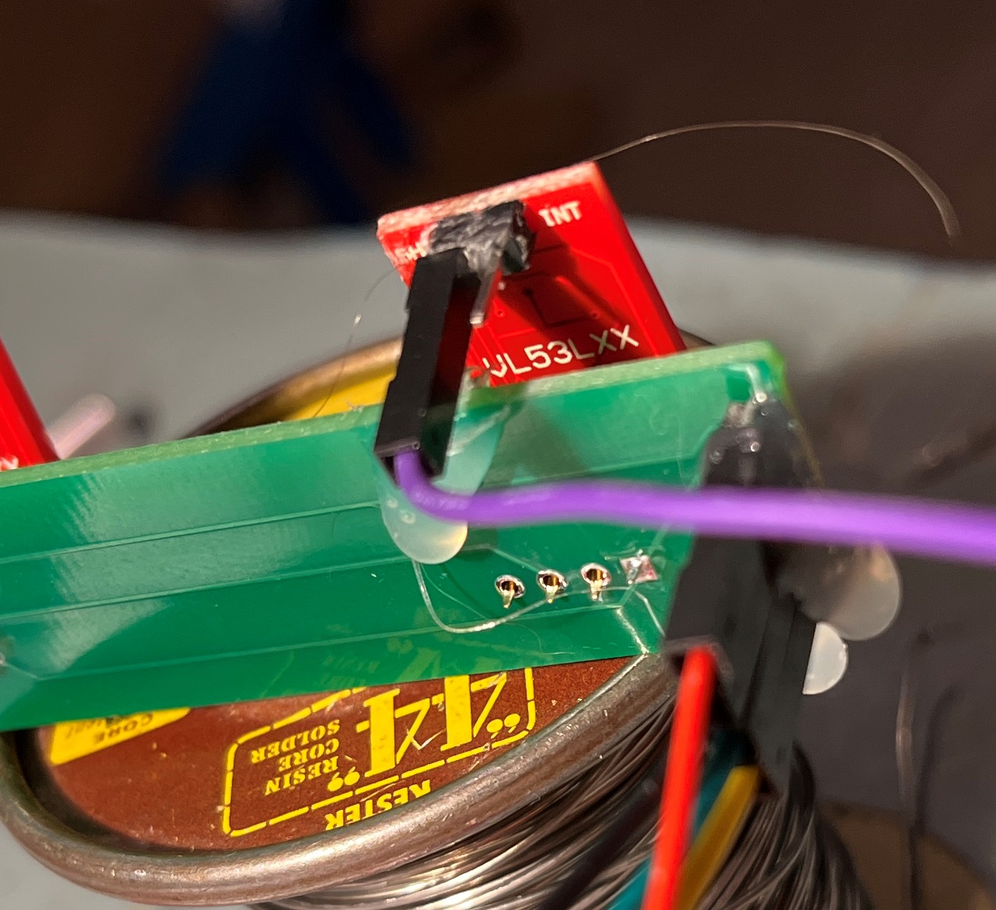
After fixing my solder (or lack thereof) screwup, everything started working – yay! Just as an aside, I claim credit for starting this troubleshooting effort with the statement “Hardware Never Fails”, which turned out to indeed be the case. Small comfort, but I’ll take it!
After confirming that both 3-element arrays were working properly, I added the rear sensor VL53L1X as a fourth sensor on Wire2, with XSHUT connected to pin 8. This mimics the hardware arrangement implemented on WallE3. Here’s a photo showing the plugboard setup:
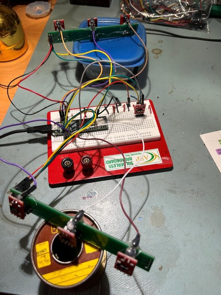
In the above image, the ‘rear’ sensor is show standing upright on the right side of the plugboard.
|
1 2 3 4 5 6 7 8 9 10 11 12 13 14 15 16 17 18 19 20 21 22 23 24 25 26 27 28 29 30 31 32 33 34 35 36 37 38 39 40 41 42 43 44 45 46 47 48 49 50 51 52 53 54 55 56 57 58 59 60 61 62 63 64 65 66 67 68 69 70 71 72 73 74 75 76 77 78 79 80 81 82 83 84 85 86 87 88 89 90 91 92 93 94 95 96 97 98 99 100 101 102 103 104 105 106 107 108 109 110 111 112 113 114 115 116 117 118 119 120 121 122 123 124 125 126 127 128 129 130 131 132 133 134 135 136 137 138 139 140 141 142 143 144 145 146 147 148 149 150 151 152 153 154 |
/* Name: VL53L1X_Pololu_V1.ino Created: 4/14/2023 4:55:00 PM Author: FRANKNEWXPS15\Frank */ /* This example shows how to set up and read multiple VL53L1X sensors connected to the same I2C bus. Each sensor needs to have its XSHUT pin connected to a different Arduino pin, and you should change sensorCount and the xshutPins array below to match your setup. For more information, see ST's application note AN4846 ("Using multiple VL53L0X in a single design"). The principles described there apply to the VL53L1X as well. 04/22/23 - this example was modified to connect three sensors (RF, RC, RR) to I2C Wire1, and four sensors (LF, LC, LR & Rear) to I2C Wire2. This mimics the hardware arrangment used on the actual robot. */ #include <Wire.h> #include <VL53L1X.h> // The number of sensors in your system. const uint8_t Wire1sensorCount = 3; //const uint8_t Wire2sensorCount = 3; const uint8_t Wire2sensorCount = 4; // The Arduino pin connected to the XSHUT pin of each sensor. const uint8_t Wire1xshutPins[Wire1sensorCount] = {23,22,21};//04/14/23 //const uint8_t Wire2xshutPins[Wire2sensorCount] = {5,6,7};//04/22/23, post soldering fix const uint8_t Wire2xshutPins[Wire2sensorCount] = {5,6,7,8};//04/22/23, post soldering fix VL53L1X Wire1sensors[Wire1sensorCount]; VL53L1X Wire2sensors[Wire2sensorCount]; void setup() { while (!Serial) {} Serial.begin(115200); delay(2000); //04/14/23 needed for Teensy Wire.begin(); Wire1.begin(); Wire2.begin(); //move some sensors to Wire1 for (uint8_t i = 0; i < Wire1sensorCount; i++) { //sensors[i].setBus(&Wire2); Wire1sensors[i].setBus(&Wire1); } for (uint8_t i = 0; i < Wire2sensorCount; i++) { //sensors[i].setBus(&Wire2); Wire2sensors[i].setBus(&Wire2); } // Disable/reset all sensors by driving their XSHUT pins low. for (uint8_t i = 0; i < Wire1sensorCount; i++) { pinMode(Wire1xshutPins[i], OUTPUT); digitalWrite(Wire1xshutPins[i], LOW); Serial.printf("Set pin %d LOW\n", Wire1xshutPins[i]); } for (uint8_t i = 0; i < Wire2sensorCount; i++) { pinMode(Wire2xshutPins[i], OUTPUT); digitalWrite(Wire2xshutPins[i], LOW); Serial.printf("Set pin %d LOW\n", Wire2xshutPins[i]); } // Enable, initialize, and start each sensor, one by one. for (uint8_t i = 0; i < Wire1sensorCount; i++) { // Stop driving this sensor's XSHUT low. This should allow the carrier // board to pull it high. (We do NOT want to drive XSHUT high since it is // not level shifted.) Then wait a bit for the sensor to start up. //pinMode(xshutPins[i], INPUT); pinMode(Wire1xshutPins[i], INPUT); Serial.printf("Set pin %d to INPUT\n", Wire1xshutPins[i]); delay(10); Wire1sensors[i].setTimeout(500); if (!Wire1sensors[i].init()) { Serial.print("Failed to detect and initialize sensor "); Serial.println(i); while (1); } else { Serial.printf("init() succeeded for sensor %d\n", i); } // Each sensor must have its address changed to a unique value other than // the default of 0x29 (except for the last one, which could be left at // the default). To make it simple, we'll just count up from 0x2A. Wire1sensors[i].setAddress(0x2A + i); Serial.printf("sensor %d I2C address set to 0X%X\n",i, Wire1sensors[i].getAddress()); Wire1sensors[i].startContinuous(50); } for (uint8_t i = 0; i < Wire2sensorCount; i++) { // Stop driving this sensor's XSHUT low. This should allow the carrier // board to pull it high. (We do NOT want to drive XSHUT high since it is // not level shifted.) Then wait a bit for the sensor to start up. //pinMode(xshutPins[i], INPUT); pinMode(Wire2xshutPins[i], INPUT); Serial.printf("Set pin %d to INPUT\n", Wire2xshutPins[i]); delay(10); Wire2sensors[i].setTimeout(500); if (!Wire2sensors[i].init()) { Serial.print("Failed to detect and initialize sensor "); Serial.println(i); while (1); } else { Serial.printf("init() succeeded for sensor %d\n", i); } // Each sensor must have its address changed to a unique value other than // the default of 0x29 (except for the last one, which could be left at // the default). To make it simple, we'll just count up from 0x2A. Wire2sensors[i].setAddress(0x2A + i); Serial.printf("sensor %d I2C address set to 0X%X\n", i, Wire2sensors[i].getAddress()); Wire2sensors[i].startContinuous(50); } } void loop() { for (uint8_t i = 0; i < Wire1sensorCount; i++) { Serial.print(Wire1sensors[i].read()); if (Wire1sensors[i].timeoutOccurred()) { Serial.print(" TIMEOUT"); } Serial.print('\t'); } for (uint8_t i = 0; i < Wire2sensorCount; i++) { Serial.print(Wire2sensors[i].read()); if (Wire2sensors[i].timeoutOccurred()) { Serial.print(" TIMEOUT"); } Serial.print('\t'); } Serial.println(); } |
And some typical output:
|
1 2 3 4 5 6 7 8 9 10 11 12 13 14 15 16 17 18 19 20 21 22 23 24 25 26 27 28 29 30 31 32 33 34 35 36 37 38 39 40 41 42 43 44 45 46 47 48 49 50 51 52 53 54 55 56 57 58 59 60 61 62 63 64 |
Opening port Port open Set pin 23 LOW Set pin 22 LOW Set pin 21 LOW Set pin 5 LOW Set pin 6 LOW Set pin 7 LOW Set pin 8 LOW Set pin 23 to INPUT init() succeeded for sensor 0 sensor 0 I2C address set to 0X2A Set pin 22 to INPUT init() succeeded for sensor 1 sensor 1 I2C address set to 0X2B Set pin 21 to INPUT init() succeeded for sensor 2 sensor 2 I2C address set to 0X2C Set pin 5 to INPUT init() succeeded for sensor 0 sensor 0 I2C address set to 0X2A Set pin 6 to INPUT init() succeeded for sensor 1 sensor 1 I2C address set to 0X2B Set pin 7 to INPUT init() succeeded for sensor 2 sensor 2 I2C address set to 0X2C Set pin 8 to INPUT init() succeeded for sensor 3 sensor 3 I2C address set to 0X2D 350 361 321 252 0 0 133 348 361 332 250 0 95 138 361 381 332 272 86 99 139 362 376 329 274 108 102 141 361 378 332 272 103 104 138 360 377 332 271 104 100 137 359 379 332 265 106 100 140 360 380 332 267 106 97 137 358 379 331 259 101 95 138 358 378 332 254 102 93 138 361 379 332 249 98 94 141 361 381 331 245 95 89 139 356 378 335 241 96 89 139 358 376 331 236 94 91 138 357 380 329 234 94 89 138 356 376 332 232 94 91 139 359 378 327 232 95 89 138 360 379 331 237 96 91 140 358 377 331 236 95 90 139 360 376 334 237 98 91 136 357 379 328 236 93 93 137 358 379 333 238 97 91 139 359 378 330 240 96 95 139 359 378 329 243 99 93 141 357 377 331 245 99 96 139 358 379 332 246 98 96 139 359 378 333 245 96 94 140 357 377 330 245 99 93 140 361 374 331 244 98 91 140 358 380 332 246 96 95 140 358 380 332 245 98 91 138 360 375 332 245 99 93 141 359 380 331 245 98 92 138 359 378 330 246 98 94 140 |
At this point I have the above ‘VL53L1X_Pololu_V1.ino’ program doing exactly what I want – handling seven different VL53L1X sensors on two different I2C busses. Now I need to port the necessary changes into my ‘Teensy_7VL53L1X_I2C_Slave_V1.ino’ program, which itself is a clone of ‘Teensy_7VL53L0X_I2C_Slave_V4.ino’, the program currently running on WallE3.
After a few minor missteps, I believe I now have ‘Teensy_7VL53L1X_I2C_Slave_V1.ino’ working with all seven VL53L1X sensors. Here’s the complete program:
|
1 2 3 4 5 6 7 8 9 10 11 12 13 14 15 16 17 18 19 20 21 22 23 24 25 26 27 28 29 30 31 32 33 34 35 36 37 38 39 40 41 42 43 44 45 46 47 48 49 50 51 52 53 54 55 56 57 58 59 60 61 62 63 64 65 66 67 68 69 70 71 72 73 74 75 76 77 78 79 80 81 82 83 84 85 86 87 88 89 90 91 92 93 94 95 96 97 98 99 100 101 102 103 104 105 106 107 108 109 110 111 112 113 114 115 116 117 118 119 120 121 122 123 124 125 126 127 128 129 130 131 132 133 134 135 136 137 138 139 140 141 142 143 144 145 146 147 148 149 150 151 152 153 154 155 156 157 158 159 160 161 162 163 164 165 166 167 168 169 170 171 172 173 174 175 176 177 178 179 180 181 182 183 184 185 186 187 188 189 190 191 192 193 194 195 196 197 198 199 200 201 202 203 204 205 206 207 208 209 210 211 212 213 214 215 216 217 218 219 220 221 222 223 224 225 226 227 228 229 230 231 232 233 234 235 236 237 238 239 240 241 242 243 244 245 246 247 248 249 250 251 252 253 254 255 256 257 258 259 260 261 262 263 264 265 266 267 268 269 270 271 272 273 274 275 276 277 278 279 280 281 282 283 284 285 286 287 288 289 290 291 292 293 294 295 296 297 298 299 300 301 302 303 304 305 306 307 308 309 310 311 312 313 314 315 316 317 318 319 320 321 322 323 324 325 326 327 328 329 330 331 332 333 334 335 336 337 338 339 340 341 342 343 344 345 346 347 348 349 350 351 352 353 354 355 356 357 358 359 360 361 362 363 364 365 366 367 368 369 370 371 372 373 374 375 376 377 378 379 380 381 382 383 384 385 386 387 388 389 390 391 392 393 394 395 396 397 398 399 400 401 402 403 404 405 406 407 408 409 410 411 412 413 414 415 416 417 418 419 420 421 422 423 424 425 426 427 428 429 430 431 432 433 434 435 436 437 438 439 440 441 442 443 444 445 446 447 448 449 450 451 452 453 454 455 456 457 458 459 460 461 462 463 464 465 466 467 468 469 470 471 472 473 474 475 476 477 478 479 480 481 482 483 484 485 486 487 488 489 490 491 492 493 494 495 496 497 498 499 500 501 502 503 504 505 506 507 508 509 510 511 512 513 514 515 516 517 518 519 520 521 522 523 524 525 526 527 528 529 530 531 532 533 534 535 536 537 538 539 540 541 542 543 544 545 546 547 548 549 550 551 552 553 554 555 556 557 558 559 560 561 562 563 564 565 566 567 568 569 570 571 572 573 574 575 576 577 578 579 580 581 582 583 584 585 586 587 588 589 590 591 592 593 594 595 596 597 598 599 600 601 602 603 604 605 606 607 608 609 610 611 612 613 614 615 616 617 618 619 620 621 622 623 624 625 626 627 628 629 630 631 632 633 634 635 636 637 638 639 640 641 642 643 644 645 646 647 648 649 650 651 652 653 654 655 656 657 658 659 660 661 662 663 664 665 666 667 668 669 670 671 672 673 674 675 676 677 678 679 680 681 682 683 684 685 686 687 688 689 690 691 692 693 694 695 696 697 698 699 700 701 702 703 704 705 706 707 708 709 710 711 712 713 714 715 716 717 718 719 720 721 722 723 724 725 726 727 728 729 730 731 732 733 |
/* Name: Teensy_7VL53L1X_I2C_Slave_V1.ino Created: 4/12/2023 3:40:21 PM Author: FRANKNEWXPS15\Frank Notes: 04/12/23 Copied from Teensy_7VL53L10X_I2C_Slave_V4 and revised to use VL53L1X sensors instead of VL53L0X, and the Pololu VL53L1X library instead of the VL53L0X one 04/21/23 code ported from VL53L1X_Pololu_V1.ino */ #pragma region EARLIER_VERSIONS /* Name: Teensy_7VL53L1X_I2C_Slave_V4.ino Created: 4/3/2022 1:04:28 PM Author: FRANKNEWXPS15\Frank Notes: 04/03/22 This version adds a linear distance correction algorithm to each VL53L1X 11/17/22 changed measurement budget from 20 to 50mSec for right-side sensors only 11/20/22 changed measurement budget from 20 to 50mSec for left-side and rear sensors 12/14/22 changed measurement budget back to 30mSec from 50mSec for all sensors */ /* Name: Teensy_7VL53L1X_I2C_Slave_V3.ino Created: 1/24/2021 4:03:35 PM Author: FRANKNEWXPS15\Frank This is the 'final' version of the Teensy 3.5 project to manage all seven VL53L1X lidar distance sensors, three on left, three on right, and now including a rear distance sensor. As of this date it was an identical copy of the TeensyHexVL53L1XHighSpeedDemo project, just renamed for clarity 01/23/22 - revised to work properly with Teensy 3.5 main processor */ /* Name: TeensyHexVL53L1XHighSpeedDemo.ino Created: 10/1/2020 3:49:01 PM Author: FRANKNEWXPS15\Frank This demo program combines the code from my Teensy_VL53L1X_I2C_Slave_V2 project with the VL53L1X 'high speed' code from the Pololu support forum post at https://forum.pololu.com/t/high-speed-with-vl53l0x/16585/3 */ /* Name: Teensy_VL53L1X_I2C_Slave_V2.ino Created: 8/4/2020 7:42:22 PM Author: FRANKNEWXPS15\Frank This project merges KurtE's multi-wire capable version of Pololu's VL53L1X library with my previous Teensy_VL53L1X_I2C_Slave project, which used the Adafruit VL53L1X library. This (hopefully) will be the version uploaded to the Teensy on the 2nd deck of Wall-E2 and which controls the left & right 3-VL53L1X sensor arrays 01/17/22: Copied VL53L1X.h/cpp from C:\Users\paynt\Documents\Arduino\Libraries\vl53l0x-arduino-multi_wire so I won't have to guess which library folder these files came from 01/17/22: if you have a local file.h same as a library\xx\file.h, then if VMicro's 'deep search'option is enabled, must use #include "file.h" instead of #include <file.h>. This is the reason for using #include "VL53L1X.h" and #include "I2C_Anything.h" below 01/17/22 the local version of "I2C_Anything.h" uses '#include <i2c_t3.h>' vice <Wire.h> for multiple I2C buss availability. 01/18/22 removed I2C_Anything.h & VL53L1X.h from project folder so can use library versions 01/22/22 added #ifdef NO_VL53L1X and assoc #ifndef blocks for debug */ #pragma endregion EARLIER_VERSIONS #include <Wire.h> //01/18/22 Wire.h has multiple I2C bus access capability #include <VL53L1X.h> #include <I2C_Anything.h> #include "elapsedMillis.h" #pragma region DEFINES //#define NO_VL53L1X #define __FILENAME__ (strrchr(__FILE__, '\\') ? strrchr(__FILE__, '\\') + 1 : __FILE__) //added 01/26/23 to extract pgm filename from full path #pragma endregion DEFINES enum VL53L1X_REQUEST { VL53L1X_READYCHECK, //added 11/10/20 to prevent bad reads during Teensy setup() VL53L1X_CENTERS_ONLY, VL53L1X_RIGHT, VL53L1X_LEFT, VL53L1X_ALL, //added 08/05/20, chg 'BOTH' to 'ALL' 10/31/20 VL53L1X_REAR_ONLY //added 10/24/20 }; #pragma region GLOBALS volatile uint8_t request_type; const int SETUP_DURATION_OUTPUT_PIN = 33; const int REQUEST_EVENT_DURATION_OUTPUT_PIN = 34; bool bTeensyReady = false; //const int MSEC_BETWEEN_LED_TOGGLES = 100; const int MSEC_BETWEEN_LED_TOGGLES = 300;//02/21/22 chg so can visually detect live I2C xfrs elapsedMillis mSecBetweenLEDToggle; //right side array uint16_t RF_Dist_mm; uint16_t RC_Dist_mm; uint16_t RR_Dist_mm; //left side array & rear uint16_t LF_Dist_mm; uint16_t LC_Dist_mm; uint16_t LR_Dist_mm; uint16_t Rear_Dist_mm; //02/20/22 back to using float for steer values float RightSteeringVal; float LeftSteeringVal; const int SLAVE_ADDRESS = 0x20; //(32Dec) just a guess for now const int DEFAULT_VL53L1X_ADDR = 0x29; //XSHUT required for I2C address init //right side array const int RF_XSHUT_PIN = 23; const int RC_XSHUT_PIN = 22; const int RR_XSHUT_PIN = 21; //left side array const int LF_XSHUT_PIN = 5; const int LC_XSHUT_PIN = 6; const int LR_XSHUT_PIN = 7; const int Rear_XSHUT_PIN = 8; //const int MAX_LIDAR_RANGE_MM = 1000; //make it obvious when nearest object is out of range const int MAX_LIDAR_RANGE_MM = 3000; //VL53L1X can go out past 3m //04/15/23 The Pololu VL53L1X library uses a parameterless constructor // and a subsequent 'setBus()' function to change the I2C bus //right side array VL53L1X lidar_RF; VL53L1X lidar_RC; VL53L1X lidar_RR; //left side array VL53L1X lidar_LF; VL53L1X lidar_LC; VL53L1X lidar_LR; //Rear sensor VL53L1X lidar_Rear; #pragma endregion GLOBALS void setup() { bTeensyReady = false; //11/10/20 prevent bad data reads by main controller Serial.begin(115200); // wait until serial port opens delay(3000); Wire.begin(SLAVE_ADDRESS); //set Teensy Wire0 port up as slave Wire.onRequest(requestEvent); //ISR for I2C requests from master (Mega 2560) Wire.onReceive(receiveEvent); //ISR for I2C data from master (Mega 2560) //initialize Wire1 & Wire2 to talk to the two arrays, plus the rear sensor Wire1.begin(); Wire2.begin(); //__FILENAME__ dynamically filled with program name Serial.printf("%lu: Starting setup() for %s\n", millis(), __FILENAME__); #pragma region PIN_INITIALIZATION pinMode(SETUP_DURATION_OUTPUT_PIN, OUTPUT); pinMode(REQUEST_EVENT_DURATION_OUTPUT_PIN, OUTPUT); pinMode(LED_BUILTIN, OUTPUT); digitalWrite(SETUP_DURATION_OUTPUT_PIN, HIGH); //right-side XSHUT control pins pinMode(RF_XSHUT_PIN, OUTPUT); pinMode(RC_XSHUT_PIN, OUTPUT); pinMode(RR_XSHUT_PIN, OUTPUT); //left-side XSHUT control pins pinMode(LF_XSHUT_PIN, OUTPUT); pinMode(LC_XSHUT_PIN, OUTPUT); pinMode(LR_XSHUT_PIN, OUTPUT); pinMode(Rear_XSHUT_PIN, OUTPUT); #pragma endregion PIN_INITIALIZATION #pragma region VL53L1X_INIT //04/15/23 The Pololu VL53L1X library uses a parameterless constructor // and a subsequent 'setBus()' function to change the I2C bus //left side array I2C SLC2/SDA2 pins 3/4 lidar_LF.setBus(&Wire2); lidar_LC.setBus(&Wire2); lidar_LR.setBus(&Wire2); lidar_Rear.setBus(&Wire2); //right side array I2C SLC1/SDA1 pins 37/38 lidar_RF.setBus(&Wire1); lidar_RC.setBus(&Wire1); lidar_RR.setBus(&Wire1); //Put all sensors in reset mode by pulling XSHUT low digitalWrite(RF_XSHUT_PIN, LOW); digitalWrite(RC_XSHUT_PIN, LOW); digitalWrite(RR_XSHUT_PIN, LOW); digitalWrite(LF_XSHUT_PIN, LOW); digitalWrite(LC_XSHUT_PIN, LOW); digitalWrite(LR_XSHUT_PIN, LOW); digitalWrite(Rear_XSHUT_PIN, LOW); //now bring lidar_RF only out of reset and set it's address //input w/o pullups sets line to high impedance so XSHUT pullup to 3.3V takes over pinMode(RF_XSHUT_PIN, INPUT); delay(10); if (!lidar_RF.init()) { Serial.println("Failed to detect and initialize lidar_RF!"); while (1) {} } //from Pololu forum post lidar_RF.setMeasurementTimingBudget(30000); //11/20/22 //lidar_RF.setMeasurementTimingBudget(50000); //11/17/22 lidar_RF.startContinuous(50); lidar_RF.setAddress(DEFAULT_VL53L1X_ADDR + 1); Serial.printf("lidar_RF address is 0x%x\n", lidar_RF.getAddress()); //now bring lidar_RC only out of reset, initialize it, and set its address //input w/o pullups sets line to high impedance so XSHUT pullup to 3.3V takes over pinMode(RC_XSHUT_PIN, INPUT); delay(10); if (!lidar_RC.init()) { Serial.println("Failed to detect and initialize lidar_RC!"); while (1) {} } //from Pololu forum post lidar_RC.setMeasurementTimingBudget(30000); //11/20/22 //lidar_RC.setMeasurementTimingBudget(50000); //11/17/22 lidar_RC.startContinuous(50); lidar_RC.setAddress(DEFAULT_VL53L1X_ADDR + 2); Serial.printf("lidar_RC address is 0x%x\n", lidar_RC.getAddress()); //now bring lidar_RR only out of reset, initialize it, and set its address //input w/o pullups sets line to high impedance so XSHUT pullup to 3.3V takes over pinMode(RR_XSHUT_PIN, INPUT); delay(10); if (!lidar_RR.init()) { Serial.println("Failed to detect and initialize lidar_RR!"); while (1) {} } //from Pololu forum post lidar_RR.setMeasurementTimingBudget(30000); //11/20/22 //lidar_RR.setMeasurementTimingBudget(50000); //11/17/22 lidar_RR.startContinuous(50); lidar_RR.setAddress(DEFAULT_VL53L1X_ADDR + 3); Serial.printf("lidar_RR address is 0x%x\n", lidar_RR.getAddress()); //now bring lidar_LF only out of reset, initialize it, and set its address //input w/o pullups sets line to high impedance so XSHUT pullup to 3.3V takes over //pinMode(LF_XSHUT_PIN, INPUT); digitalWrite(LF_XSHUT_PIN, HIGH); //Serial.printf("lidar_LF LF_XSHUT_PIN now reads %d\n", digitalRead(LF_XSHUT_PIN)); delay(10); if (!lidar_LF.init()) { Serial.println("Failed to detect and initialize lidar_LF!"); //while (1) {} } //from Pololu forum post lidar_LF.setMeasurementTimingBudget(30000); //lidar_LF.setMeasurementTimingBudget(50000); //11/20/22 lidar_LF.startContinuous(50); lidar_LF.setAddress(DEFAULT_VL53L1X_ADDR + 4); Serial.printf("lidar_LF address is 0x%x\n", lidar_LF.getAddress()); //now bring lidar_LC only out of reset, initialize it, and set its address //input w/o pullups sets line to high impedance so XSHUT pullup to 3.3V takes over pinMode(LC_XSHUT_PIN, INPUT); delay(10); if (!lidar_LC.init()) { Serial.println("Failed to detect and initialize lidar_LC!"); while (1) {} } //from Pololu forum post lidar_LC.setMeasurementTimingBudget(30000); //lidar_LC.setMeasurementTimingBudget(50000); //11/20/22 lidar_LC.startContinuous(50); lidar_LC.setAddress(DEFAULT_VL53L1X_ADDR + 5); Serial.printf("lidar_LC address is 0x%x\n", lidar_LC.getAddress()); //now bring lidar_LR only out of reset, initialize it, and set its address //input w/o pullups sets line to high impedance so XSHUT pullup to 3.3V takes over pinMode(LR_XSHUT_PIN, INPUT); if (!lidar_LR.init()) { Serial.println("Failed to detect and initialize lidar_LR!"); while (1) {} } //from Pololu forum post lidar_LR.setMeasurementTimingBudget(30000); //lidar_LR.setMeasurementTimingBudget(50000); //11/20/22 lidar_LR.startContinuous(50); lidar_LR.setAddress(DEFAULT_VL53L1X_ADDR + 6); Serial.printf("lidar_LR address is 0x%x\n", lidar_LR.getAddress()); //added 10/23/20 for rear sensor //now bring lidar_Rear only out of reset, initialize it, and set its address //input w/o pullups sets line to high impedance so XSHUT pullup to 3.3V takes over pinMode(Rear_XSHUT_PIN, INPUT); if (!lidar_Rear.init()) { Serial.println("Failed to detect and initialize lidar_Rear!"); //while (1) {} } //from Pololu forum post lidar_Rear.setMeasurementTimingBudget(30000); //lidar_Rear.setMeasurementTimingBudget(50000); //11/20/22 lidar_Rear.startContinuous(50); lidar_Rear.setAddress(DEFAULT_VL53L1X_ADDR + 7); Serial.printf("lidar_Rear address is 0x%x\n", lidar_Rear.getAddress()); #pragma endregion VL53L1X_INIT digitalWrite(SETUP_DURATION_OUTPUT_PIN, LOW); bTeensyReady = true; //11/10/20 added to prevent bad data reads by main controller mSecBetweenLEDToggle = 0; Serial.printf("Msec\tLFront\tLCtr\tLRear\tRFront\tRCtr\tRRear\tRear\tLSteer\tRSteer\n"); } void loop() { //04/03/22 now using a per-unit correction algorithm RF_Dist_mm = lidar_RF_Correction(lidar_RF.readRangeContinuousMillimeters()); RC_Dist_mm = lidar_RC_Correction(lidar_RC.readRangeContinuousMillimeters()); RR_Dist_mm = lidar_RR_Correction(lidar_RR.readRangeContinuousMillimeters()); RightSteeringVal = (RF_Dist_mm - RR_Dist_mm) / 100.f; //rev 06/21/20 see PPalace post //from Pololu forum post //LF_Dist_mm = lidar_LF.readRangeContinuousMillimeters(); //LC_Dist_mm = lidar_LC.readRangeContinuousMillimeters(); //LR_Dist_mm = lidar_LR.readRangeContinuousMillimeters(); //04/03/22 now using a per-unit correction algorithm LF_Dist_mm = lidar_LF_Correction(lidar_LF.readRangeContinuousMillimeters()); LC_Dist_mm = lidar_LC_Correction(lidar_LC.readRangeContinuousMillimeters()); LR_Dist_mm = lidar_LR_Correction(lidar_LR.readRangeContinuousMillimeters()); LeftSteeringVal = (LF_Dist_mm - LR_Dist_mm) / 100.f; //rev 06/21/20 see PPalace post //added 10/23/20 for rear sensor //Rear_Dist_mm = lidar_Rear.readRangeContinuousMillimeters(); Rear_Dist_mm = lidar_Rear_Correction(lidar_Rear.readRangeContinuousMillimeters()); if (mSecBetweenLEDToggle <= MSEC_BETWEEN_LED_TOGGLES) { mSecBetweenLEDToggle -= MSEC_BETWEEN_LED_TOGGLES; //digitalToggle(LED_BUILTIN); Serial.printf("%lu\t%d\t%d\t%d\t%d\t%d\t%d\t%d\t%2.2f\t%2.2f\n", millis(), LF_Dist_mm, LC_Dist_mm, LR_Dist_mm, RF_Dist_mm, RC_Dist_mm, RR_Dist_mm, Rear_Dist_mm, LeftSteeringVal, RightSteeringVal); } } void requestEvent() { //Purpose: Send requested sensor data to the Mega controller via main I2C bus //Inputs: // request_type = uint8_t value denoting type of data requested (from receiveEvent()) // 0 = left & right center distances only // 1 = right side front, center and rear distances, plus steering value // 2 = left side front, center and rear distances, plus steering value // 3 = both side front, center and rear distances, plus both steering values //Outputs: // Requested data sent to master //Notes: // 08/05/20 added VL53L1X_ALL request type to get both sides at once // 10/24/20 added VL53L1X_REAR_ONLY request type // 11/09/20 added write to pin for O'scope monitoring //DEBUG!! //int data_size = 0; //DEBUG!! //DEBUG!! //Serial.printf("RequestEvent() with request_type = %d: VL53L0X Front/Center/Rear distances = %d, %d, %d\n", // request_type, RF_Dist_mm, RC_Dist_mm, RR_Dist_mm); //DEBUG!! //digitalWrite(LED_BUILTIN, HIGH);//added 01/22/22 digitalWrite(REQUEST_EVENT_DURATION_OUTPUT_PIN, HIGH); digitalToggle(LED_BUILTIN);//2/21/22 added for visual indication of I2C activity switch (request_type) { case VL53L1X_READYCHECK: //added 11/10/20 to prevent bad reads during Teensy setup() Serial.printf("in VL53L1X_READYCHECK case at %lu with bTeensyReady = %d\n", millis(), bTeensyReady); I2C_writeAnything(bTeensyReady); break; case VL53L1X_CENTERS_ONLY: //DEBUG!! //data_size = 2*sizeof(uint16_t); //Serial.printf("Sending %d bytes LC_Dist_mm = %d, RC_Dist_mm = %d to master\n", data_size, LC_Dist_mm, RC_Dist_mm); //DEBUG!! I2C_writeAnything(RC_Dist_mm); I2C_writeAnything(LC_Dist_mm); break; case VL53L1X_RIGHT: //DEBUG!! //data_size = 3 * sizeof(uint16_t) + sizeof(float); //Serial.printf("Sending %d bytes RF/RC/RR/RS vals = %d, %d, %d, %3.2f to master\n", // data_size, RF_Dist_mm, RC_Dist_mm, RR_Dist_mm, RightSteeringVal); //DEBUG!! I2C_writeAnything(RF_Dist_mm); I2C_writeAnything(RC_Dist_mm); I2C_writeAnything(RR_Dist_mm); I2C_writeAnything(RightSteeringVal); break; case VL53L1X_LEFT: //DEBUG!! //data_size = 3 * sizeof(uint16_t) + sizeof(float); //Serial.printf("Sending %d bytes LF/LC/LR/LS vals = %d, %d, %d, %3.2f to master\n", // data_size, LF_Dist_mm, LC_Dist_mm, LR_Dist_mm, LeftSteeringVal); //DEBUG!! I2C_writeAnything(LF_Dist_mm); I2C_writeAnything(LC_Dist_mm); I2C_writeAnything(LR_Dist_mm); I2C_writeAnything(LeftSteeringVal); break; case VL53L1X_ALL: //Serial.printf("In VL53L1X_ALL case\n"); //added 08/05/20 to get data from both sides at once //10/31/20 chg to VL53L1X_ALL & report all 7 sensor values //DEBUG!! //data_size = 3 * sizeof(uint16_t) + sizeof(float); //data_size = 7 * sizeof(uint16_t) + 2 * sizeof(float); //Serial.printf("Sending %d bytes to master\n", data_size); //Serial.printf("%d bytes: %d\t%d\t%d\t%3.2f\t%d\t%d\t%d\t%d\t%3.2f\n", // data_size, LF_Dist_mm, LC_Dist_mm, LR_Dist_mm, LeftSteeringVal, // RF_Dist_mm, RC_Dist_mm, RR_Dist_mm, Rear_Dist_mm, RightSteeringVal); //DEBUG!! //DEBUG!! //data_size = 3 * sizeof(uint16_t) + sizeof(float); //Serial.printf("Sending %d bytes LF/LC/LR/LS vals = %d, %d, %d, %3.2f to master\n", // data_size, LF_Dist_mm, LC_Dist_mm, LR_Dist_mm, LeftSteeringVal); //DEBUG!! //left side I2C_writeAnything(LF_Dist_mm); I2C_writeAnything(LC_Dist_mm); I2C_writeAnything(LR_Dist_mm); I2C_writeAnything(LeftSteeringVal); //DEBUG!! //data_size = 3 * sizeof(uint16_t) + sizeof(float); //data_size = 4 * sizeof(uint16_t) + sizeof(float); //Serial.printf("Sending %d bytes RF/RC/RR/R/RS vals = %d, %d, %d, %d, %3.2f to master\n", // data_size, RF_Dist_mm, RC_Dist_mm, RR_Dist_mm, Rear_Dist_mm, RightSteeringVal); //DEBUG!! //right side I2C_writeAnything(RF_Dist_mm); I2C_writeAnything(RC_Dist_mm); I2C_writeAnything(RR_Dist_mm); I2C_writeAnything(Rear_Dist_mm); I2C_writeAnything(RightSteeringVal); break; case VL53L1X_REAR_ONLY: //DEBUG!! //data_size = sizeof(uint16_t); //Serial.printf("Sending %d bytes Rear_Dist_mm = %d to master\n", data_size, Rear_Dist_mm); //DEBUG!! I2C_writeAnything(Rear_Dist_mm); break; default: break; } digitalToggle(LED_BUILTIN);//2/21/22 added for visual indication of I2C activity digitalWrite(REQUEST_EVENT_DURATION_OUTPUT_PIN, LOW); //digitalWrite(LED_BUILTIN, LOW);//added 01/22/22 } void receiveEvent(int numBytes) { //Purpose: capture data request type from Mega I2C master //Inputs: // numBytes = int value denoting number of bytes received from master //Outputs: // uint8_t request_type filled with request type value from master //DEBUG!! //Serial.printf("receiveEvent(%d)\n", numBytes); //DEBUG!! I2C_readAnything(request_type); //DEBUG!! //Serial.printf("receiveEvent: Got %d from master\n", request_type); //DEBUG!! } uint16_t lidar_LF_Correction(uint16_t raw_dist) { //Purpose: Correct for linear error in left front VL53L0X //Provenance: Created 04/03/22 gfp //Inputs: // raw_dist = uint16_t value denoting raw measurement in mm //Outputs: // returns raw_dist (mm) corrected for linear distance measurement error //Notes: // correction = =(raw + 0.4)/1.125 // 04/05/22 bugfix. Raw dist here are MM, but above formula assumed CM - fixed below // correction = =(raw(mm) + 4)/1.125 //uint16_t corrVal = (uint16_t)((float)raw_dist + 0.4f) / 1.125f; //uint16_t corrVal = (uint16_t)((float)raw_dist + 4.f) / 1.125f; //uint16_t corrVal = raw_dist; uint16_t corrVal = (uint16_t)((float)raw_dist - 5.478f) / 1.0918f;//11/20/22 //DEBUG!! //Serial.printf("LF: raw = %d, corr = %d\n", raw_dist, corrVal); //DEBUG!! return corrVal; } uint16_t lidar_LC_Correction(uint16_t raw_dist) { //Purpose: Correct for linear error in left center VL53L0X //Provenance: Created 04/03/22 gfp //Inputs: // raw_dist = uint16_t value denoting raw measurement in mm //Outputs: // returns raw_dist corrected for linear distance measurement error //Notes: // correction = ==(raw - 0.6333)/1.03 // 04/05/22 bugfix. Raw dist here are MM, but above formula assumed CM - fixed below // correction = =(raw(mm) - 6.333)/1.03 //uint16_t corrVal = (uint16_t)((float)raw_dist - 0.6333f) / 1.03f; //uint16_t corrVal = (uint16_t)((float)raw_dist - 6.333f) / 1.03f; //uint16_t corrVal = raw_dist; uint16_t corrVal = (uint16_t)((float)raw_dist - 19.89f) / 0.9913f;//11/20/22 //DEBUG!! //Serial.printf("LC: raw = %d, corr = %d\n", raw_dist, corrVal); //DEBUG!! return corrVal; } uint16_t lidar_LR_Correction(uint16_t raw_dist) { //Purpose: Correct for linear error in left rear VL53L0X //Provenance: Created 04/03/22 gfp //Inputs: // raw_dist = uint16_t value denoting raw measurement in mm //Outputs: // returns raw_dist corrected for linear distance measurement error //Notes: // correction = =raw - 2.0667 // 04/05/22 bugfix. Raw dist here are MM, but above formula assumed CM - fixed below // correction = = raw(mm) - 20.667 //uint16_t corrVal = (uint16_t)((float)raw_dist - 2.0667f); //uint16_t corrVal = (uint16_t)((float)raw_dist - 20.667f); //uint16_t corrVal = raw_dist; uint16_t corrVal = (uint16_t)((float)raw_dist + 9.676f) / 1.1616; //DEBUG!! //Serial.printf("LR: raw = %d, corr = %d\n", raw_dist, corrVal); //DEBUG!! return corrVal; } uint16_t lidar_RF_Correction(uint16_t raw_dist) { //Purpose: Correct for linear error in right front VL53L0X //Provenance: Created 04/03/22 gfp //Inputs: // raw_dist = uint16_t value denoting raw measurement in mm //Outputs: // returns raw_dist corrected for linear distance measurement error in mm //Notes: // correction = =(raw + 0.96)/1.045 // 04/05/22 bugfix. Raw dist here are MM, but above formula assumed CM - fixed below // correction = =(raw(mm) + 9.6f)/1.03f //uint16_t corrVal = (uint16_t)((float)raw_dist + 0.96f) / 1.045f; //uint16_t corrVal = (uint16_t)((float)raw_dist + 9.6f) / 1.045f; //uint16_t corrVal = raw_dist; //11/18/22 uint16_t corrVal = (uint16_t)((float)raw_dist - 4.297f) / 1.0808f; //DEBUG!! //Serial.printf("RF: raw = %d, corr = %d\n", raw_dist, corrVal); //DEBUG!! return corrVal; } uint16_t lidar_RC_Correction(uint16_t raw_dist) { //Purpose: Correct for linear error in right center VL53L0X //Provenance: Created 04/03/22 gfp //Inputs: // raw_dist = uint16_t value denoting raw measurement in mm //Outputs: // returns raw_dist corrected for linear distance measurement error //Notes: // correction = =(raw - 3.2)/1.08 // 04/05/22 bugfix. Raw dist here are MM, but above formula assumed CM - fixed below // correction = =(raw(mm) - 3.2)/1.08 //uint16_t corrVal = (uint16_t)((float)raw_dist - 3.2f) / 1.08f; //uint16_t corrVal = (uint16_t)((float)raw_dist - 32.f) / 1.08f; //uint16_t corrVal = raw_dist; uint16_t corrVal = (uint16_t)((float)raw_dist - 50.603f) / 1.0438f; //DEBUG!! //Serial.printf("RC: raw = %d, corr = %d\n", raw_dist, corrVal); //DEBUG!! return corrVal; } uint16_t lidar_RR_Correction(uint16_t raw_dist) { //Purpose: Correct for linear error in right rear VL53L0X //Provenance: Created 04/03/22 gfp //Inputs: // raw_dist = uint16_t value denoting raw measurement in mm //Outputs: // returns raw_dist corrected for linear distance measurement error //Notes: // correction = =(raw - 3.1)/1.12 // 04/05/22 bugfix. Raw dist here are MM, but above formula assumed CM - fixed below // correction = =(raw(mm) - 31)/1.12 //uint16_t corrVal = (uint16_t)((float)raw_dist - 3.1f) / 1.12f; //uint16_t corrVal = (uint16_t)((float)raw_dist - 31.f) / 1.12f; //uint16_t corrVal = raw_dist; uint16_t corrVal = (uint16_t)((float)raw_dist - 56.746f) / 1.0353; //DEBUG!! //Serial.printf("RR: raw = %d, corr = %d\n", raw_dist, corrVal); //DEBUG!! return corrVal; } uint16_t lidar_Rear_Correction(uint16_t raw_dist) { //Purpose: Correct for linear error in rear VL53L0X //Provenance: Created 04/03/22 gfp //Inputs: // raw_dist = uint16_t value denoting raw measurement in mm //Outputs: // returns raw_dist corrected for linear distance measurement error //Notes: // correction = ==(raw - 1.1)/1.09 // 04/05/22 bugfix. Raw dist here are MM, but above formula assumed CM - fixed below // correction = =(raw(mm) - 11)/1.09 //uint16_t corrVal = (uint16_t)((float)raw_dist - 1.1f) / 1.09f; uint16_t corrVal = (uint16_t)((float)raw_dist - 11.f) / 1.09f; //DEBUG!! //Serial.printf("Rear: raw = %d, corr = %d\n", raw_dist, corrVal); //DEBUG!! return corrVal; } |
And a sample of the output:
|
1 2 3 4 5 6 7 8 9 10 11 12 13 14 15 16 17 18 19 20 21 22 23 24 25 26 27 28 29 30 31 32 33 34 35 36 37 38 39 40 41 42 43 44 45 46 47 48 49 50 51 52 53 54 55 56 57 58 59 60 61 62 63 64 65 66 67 |
Opening port Port open 3300: Starting setup() for Teensy_7VL53L1X_I2C_Slave_V1.ino lidar_RF address is 0x2a lidar_RC address is 0x2b lidar_RR address is 0x2c lidar_LF address is 0x2d lidar_LC address is 0x2e lidar_LR address is 0x2f lidar_Rear address is 0x30 Msec LFront LCtr LRear RFront RCtr RRear Rear LSteer RSteer 3607 361 249 274 322 263 251 107 0.87 0.71 3871 366 267 287 346 282 263 114 0.79 0.83 4197 368 269 283 329 280 269 115 0.85 0.60 4476 368 268 292 330 279 261 113 0.76 0.69 4756 371 269 284 332 282 262 113 0.87 0.70 5083 372 273 303 333 279 263 114 0.69 0.70 5362 368 271 287 331 280 260 111 0.81 0.71 5688 376 281 285 327 283 262 115 0.91 0.65 5968 369 276 305 341 289 262 113 0.64 0.79 6294 368 274 288 331 279 266 112 0.80 0.65 6574 375 292 303 327 282 263 114 0.72 0.64 6900 415 338 334 322 283 263 114 0.81 0.59 7180 427 359 347 329 282 261 110 0.80 0.68 7459 434 367 351 332 280 259 116 0.83 0.73 7785 69 46 350 328 287 262 113 -2.81 0.66 8065 16 18 35 331 279 258 115 -0.19 0.73 8392 9 8 33 322 284 263 114 -0.24 0.59 8674 6 7 17 321 286 265 112 -0.11 0.56 8955 0 0 7 323 284 263 111 -0.07 0.60 9283 0 0 7 348 277 266 112 -0.07 0.82 9565 0 0 8 339 285 267 111 -0.08 0.72 9894 4 0 9 327 283 261 111 -0.05 0.66 10175 422 0 8 326 280 261 115 4.14 0.65 10457 438 0 7 323 287 260 114 4.31 0.63 10785 436 0 7 321 286 262 114 4.29 0.59 11066 386 0 7 322 286 264 117 3.79 0.58 11394 435 0 7 346 285 263 121 4.28 0.83 11676 438 0 7 321 284 264 117 4.31 0.57 11960 19 0 7 322 282 261 114 0.12 0.61 12291 450 72 39 321 284 266 112 4.11 0.55 12575 448 395 348 325 288 264 138 1.00 0.61 12900 443 395 341 321 286 260 136 1.02 0.61 13179 440 388 334 322 282 261 125 1.06 0.61 13459 435 385 326 321 281 264 166 1.09 0.57 13787 435 380 323 325 283 260 0 1.12 0.65 14078 428 380 325 321 289 260 24 1.03 0.61 14357 434 391 324 321 287 263 0 1.10 0.58 14684 434 388 327 324 286 261 1 1.07 0.63 14963 436 382 330 325 285 263 35 1.06 0.62 15289 433 388 332 322 286 265 12 1.01 0.57 15569 437 394 334 322 286 264 116 1.03 0.58 15898 437 388 329 327 286 263 115 1.08 0.64 16179 428 383 331 321 284 263 116 0.97 0.58 16460 427 387 335 323 285 269 114 0.92 0.54 16789 433 387 334 322 286 261 114 0.99 0.61 17070 428 396 331 321 284 259 117 0.97 0.62 17399 430 386 327 321 283 263 111 1.03 0.58 17683 416 385 311 323 284 260 114 1.05 0.63 17963 408 385 310 323 289 264 117 0.98 0.59 18290 403 375 315 323 288 261 115 0.88 0.62 18571 387 377 307 326 284 264 115 0.80 0.62 18900 360 361 275 323 263 262 113 0.85 0.61 19181 315 385 336 321 11 28 114 -0.21 2.93 19463 305 404 379 18 0 0 113 -0.74 0.18 19791 307 412 401 11 0 0 115 -0.94 0.11 20072 316 415 407 236 0 0 113 -0.91 2.36 |
At this point the only remaining step is to physically swap out the sensors currently on WallE3 with the new ones, and reprogram the 2nd deck Teensy 3.5 with the new ‘Teensy_7VL53L1X_I2C_Slave_V1.ino’. With any luck at all, WallE3 won’t even notice anything has changed, except he will now be getting valid side/rear distance values from much farther away. We’ll see!
26 April 2023 Update:
After carefully installing all seven sensors (two 3-element arrays plus a rear-facing one) on WallE3’s second deck, and running the same Pololu example program on the second-deck Teensy 3.5, I discovered that one of the sensors was initializing properly, but was reporting ‘0 TIMEOUT’ for the distance – major bummer! After removing the left-hand sensor array from WallE3 and re-attaching it to my free-standing test Teensy 3.5, I eventually found that the problem was a broken connection INSIDE one of the 4-pin female headers on the PCB – yikes!
Anyway, got that fixed, re-attached the left-hand array to WallE3, and ran the Pololu program to verify proper operation, and now all seven element report believable distances, as shown below. In the output below, I used my hand to block the right, left, and rear sensors to verify proper performance.
|
1 2 3 4 5 6 7 8 9 10 11 12 13 14 15 16 17 18 19 20 21 22 23 24 25 26 27 28 29 30 31 32 33 34 35 36 37 38 39 40 41 42 43 44 45 46 47 48 49 50 51 52 53 54 55 56 57 58 59 60 61 62 63 64 65 66 67 68 69 70 71 72 73 74 75 76 77 78 79 80 81 82 83 84 85 86 87 88 89 90 91 92 93 94 95 96 97 98 99 100 101 102 103 104 105 106 107 108 109 110 111 112 113 114 115 116 117 118 119 120 121 122 123 124 125 126 127 128 129 130 131 132 133 134 135 136 137 138 139 140 141 142 143 144 |
Opening port Port open Set pin 23 LOW Set pin 22 LOW Set pin 21 LOW Set pin 23 to INPUT init() succeeded for sensor 0 sensor 0 I2C address set to 0X2A Set pin 22 to INPUT init() succeeded for sensor 1 sensor 1 I2C address set to 0X2B Set pin 21 to INPUT init() succeeded for sensor 2 sensor 2 I2C address set to 0X2C Set pin 5 LOW Set pin 6 LOW Set pin 7 LOW Set pin 8 LOW Set pin 5 to INPUT init() succeeded for sensor 0 sensor 0 I2C address set to 0X2A Set pin 6 to INPUT init() succeeded for sensor 1 sensor 1 I2C address set to 0X2B Set pin 7 to INPUT init() succeeded for sensor 2 sensor 2 I2C address set to 0X2C Set pin 8 to INPUT init() succeeded for sensor 3 sensor 3 I2C address set to 0X2D 2615 302 346 351 378 480 482 2253 2685 300 346 368 377 482 485 2252 2763 316 359 371 389 492 486 2257 2856 314 360 373 387 489 481 2245 2949 312 360 372 386 489 484 2266 3042 316 358 370 387 489 485 2260 3136 314 363 373 385 492 485 2257 3228 316 359 372 383 491 482 2254 3322 317 360 369 387 491 484 2251 3415 317 360 370 388 490 484 2260 3508 315 357 371 386 488 483 2266 3601 315 358 369 386 490 483 2260 3694 312 358 373 385 490 483 2253 3788 314 359 370 386 490 481 2267 3880 316 359 371 387 488 483 2258 3974 315 362 371 383 488 483 2250 4067 316 363 370 387 488 480 2257 4160 313 364 373 384 486 480 2257 4253 315 361 371 382 486 480 2252 4346 316 360 368 383 485 477 2256 4440 316 359 375 383 488 480 2256 4532 319 361 370 383 489 481 2263 4626 314 362 373 386 491 481 2262 4719 317 361 371 390 495 487 2260 4812 315 363 367 391 497 487 2254 4905 313 358 367 396 497 490 2246 4998 316 356 372 397 495 490 2252 5091 315 361 372 398 499 493 2258 5184 314 357 370 401 502 498 2249 5278 316 362 371 400 501 494 2265 5371 318 357 371 400 501 491 2263 5464 313 360 367 399 503 497 2258 5557 313 362 368 401 506 503 2252 5650 315 362 371 404 510 500 2250 5743 311 361 370 412 517 500 2254 5836 314 360 368 410 516 494 2256 5929 315 360 371 408 497 485 2261 6023 314 361 370 407 471 482 2262 6116 316 361 370 408 456 477 2253 6209 315 357 368 421 443 477 2254 6302 316 359 373 437 453 483 2251 6395 314 360 371 454 442 485 2257 6489 316 358 368 441 381 422 2252 6581 317 355 370 253 412 231 2250 6675 314 362 370 482 541 496 2248 6768 316 359 372 501 564 506 1559 6861 312 360 370 509 573 520 44 6954 315 362 372 510 578 526 97 7048 316 362 370 510 576 524 86 7141 317 362 373 502 575 521 73 7234 317 359 373 498 578 520 67 7328 317 360 368 505 578 515 61 7420 315 361 371 500 577 508 53 7514 315 360 371 499 576 504 52 7607 319 358 372 505 578 503 55 7700 318 361 372 502 576 510 67 7793 317 362 372 503 576 496 104 7886 313 360 370 499 564 458 2265 7954 323 357 369 489 516 399 2257 8032 316 360 367 471 445 367 2265 8125 315 362 371 451 421 397 2256 8218 315 359 372 399 405 404 2251 8311 315 359 372 374 403 405 2264 8405 315 360 374 370 415 403 2260 8497 317 357 370 373 420 406 2245 8591 315 360 372 379 415 412 2260 8683 314 361 375 374 420 415 2255 8777 315 360 371 376 414 413 2262 8869 314 359 370 370 409 415 2255 8963 313 359 373 368 412 426 2252 9055 316 357 371 359 395 453 2260 9149 318 358 369 323 390 470 2258 9242 314 361 374 259 374 467 2256 9334 314 361 370 205 355 465 2257 9428 314 359 369 157 357 455 2250 9520 316 359 371 109 379 464 2242 9614 315 359 369 62 119 116 2256 9706 314 362 374 39 0 2 2256 9799 313 360 371 31 2 6 2253 9893 314 359 373 24 0 5 2255 9985 315 358 371 21 1 4 2250 10079 315 361 374 19 1 3 2257 10171 314 358 369 21 0 6 2261 10265 317 360 369 20 0 3 2253 10357 316 360 371 21 1 4 2263 10451 315 359 376 19 1 5 2259 10544 316 357 372 23 1 7 2261 10637 318 361 371 37 4 1072 2256 10726 317 360 369 243 1221 1251 2255 10820 320 360 371 408 1130 460 2262 10913 315 360 372 432 437 468 2255 11006 317 357 373 447 450 477 2258 11100 316 359 372 462 465 482 2260 11195 316 358 372 469 467 480 2257 11288 318 358 371 466 468 472 2256 11381 315 360 369 460 461 462 2250 11474 315 358 370 448 452 455 2268 11567 316 355 372 439 444 442 2249 11661 313 355 371 431 441 434 2251 11755 316 361 371 422 436 424 2258 11848 319 356 372 408 428 414 2263 11942 315 357 370 391 424 403 2260 12036 236 360 369 379 415 388 2253 12130 0 40 370 372 414 383 2256 12223 5 1 372 365 410 382 2269 12317 10 5 370 365 408 383 2266 12411 5 3 371 369 413 379 2260 12505 2 0 277 368 409 381 2246 12598 28 0 314 368 413 381 2264 12692 15 4 0 372 413 383 2260 12786 8 1 277 367 414 385 2255 12880 167 54 539 372 418 388 2260 12973 319 530 369 372 418 389 2254 13067 315 359 371 375 420 392 2262 |
Next, I loaded my new ‘Teensy_7VL53L1X_I2C_Slave_V1.ino’ program on WallE3’s second-deck Teensy 3.5 and verified that all seven sensors were operating properly, as shown in the output below:
|
1 2 3 4 5 6 7 8 9 10 11 12 13 14 15 16 17 18 19 20 21 22 23 24 25 26 27 28 29 30 31 32 33 34 35 36 37 38 39 40 41 42 43 44 45 46 47 48 49 50 51 52 53 54 55 56 57 58 59 60 61 62 63 64 65 66 67 68 69 70 71 72 73 74 75 76 77 78 79 80 81 82 83 84 85 86 87 88 89 90 91 92 93 94 95 96 97 98 99 |
Opening port Port open 3300: Starting setup() for Teensy_7VL53L1X_I2C_Slave_V1.ino lidar_RF address is 0x2a lidar_RC address is 0x2b lidar_RR address is 0x2c lidar_LF address is 0x2d lidar_LC address is 0x2e lidar_LR address is 0x2f lidar_Rear address is 0x30 Msec LFront LCtr LRear RFront RCtr RRear Rear LSteer RSteer 3605 481 573 525 282 259 243 766 -0.44 0.39 3869 478 570 519 303 277 265 762 -0.41 0.38 4197 472 565 516 307 282 267 768 -0.44 0.40 4476 470 565 517 309 277 262 762 -0.47 0.47 4755 475 568 523 309 277 266 766 -0.48 0.43 5083 472 563 516 306 274 260 766 -0.44 0.46 5365 434 524 498 305 276 259 762 -0.64 0.46 5693 264 707 575 305 277 266 768 -3.11 0.39 5976 181 890 600 304 275 259 766 -4.19 0.45 6256 136 2995 688 305 280 262 767 -5.52 0.43 6588 113 3011 1152 303 275 258 769 -10.39 0.45 6867 116 3036 914 303 280 258 766 -7.98 0.45 7195 134 2420 669 305 279 263 777 -5.35 0.42 7478 122 1863 746 307 277 264 778 -6.24 0.43 7758 119 2323 891 306 278 262 771 -7.72 0.44 8087 125 2748 655 303 275 263 762 -5.30 0.40 8368 114 2842 701 303 277 260 772 -5.87 0.43 8697 124 2664 792 301 275 260 767 -6.68 0.41 8979 122 2994 743 308 278 260 763 -6.21 0.48 9262 119 2857 782 309 277 257 775 -6.63 0.52 9588 130 2356 878 306 277 261 777 -7.48 0.45 9870 122 2816 1003 302 277 258 767 -8.81 0.44 10199 117 2709 907 303 281 263 770 -7.90 0.40 10496 120 3053 799 306 278 259 770 -6.79 0.47 10776 115 2635 659 307 280 260 771 -5.44 0.47 11055 119 2404 792 301 275 258 766 -6.73 0.43 11378 116 2653 902 300 277 260 766 -7.86 0.40 11659 119 3189 658 305 277 258 766 -5.39 0.47 11985 124 2693 659 303 278 263 762 -5.35 0.40 12264 129 2542 805 305 278 257 765 -6.76 0.48 12593 130 2739 789 311 278 264 770 -6.59 0.47 12873 121 2645 1509 304 273 259 774 -13.88 0.45 13155 116 2496 983 306 278 260 767 -8.67 0.46 13483 128 3174 838 306 276 262 771 -7.10 0.44 13765 127 2526 760 305 277 262 762 -6.33 0.43 14093 127 2531 757 304 274 261 767 -6.30 0.43 14375 120 2757 758 307 275 267 764 -6.38 0.40 14656 131 2780 888 309 275 262 762 -7.57 0.47 14987 130 2540 620 302 275 266 766 -4.90 0.36 15266 0 2503 720 309 277 265 763 -7.20 0.44 15568 33 0 18 308 278 267 772 0.15 0.41 15893 30 0 14 297 277 268 785 0.16 0.29 16173 28 0 12 304 281 263 792 0.16 0.41 16498 30 0 11 309 277 269 802 0.19 0.40 16777 34 0 12 304 273 271 802 0.22 0.33 17057 28 0 7 304 278 267 781 0.21 0.37 17382 23 0 7 310 274 263 787 0.16 0.47 17661 24 0 9 304 277 268 776 0.15 0.36 17987 19 0 7 301 280 263 783 0.12 0.38 18269 11 0 8 307 279 261 781 0.03 0.46 18597 9 0 8 304 276 260 780 0.01 0.44 18879 10 0 10 306 280 261 777 0.00 0.45 19160 13 0 8 305 284 262 779 0.05 0.43 19489 184 91 75 305 280 259 766 1.09 0.46 19774 246 192 125 302 277 258 0 1.21 0.44 20099 243 182 153 308 274 264 0 0.90 0.44 20380 254 188 154 307 277 266 0 1.00 0.41 20662 262 199 165 307 279 254 0 0.97 0.53 20992 264 202 173 309 276 260 0 0.91 0.49 21272 272 204 173 305 277 262 0 0.99 0.43 21601 270 218 167 306 275 265 8 1.03 0.41 21882 191 2948 238 303 281 258 775 -0.47 0.45 22164 45 2703 2574 254 20 136 766 -25.29 1.18 22492 41 3237 2540 0 0 0 765 -24.99 0.00 22774 36 3147 2267 0 0 0 759 -22.31 0.00 23058 40 3097 2679 0 0 0 766 -26.39 0.00 23384 40 3175 2506 0 0 0 771 -24.66 0.00 23669 29 3409 2853 0 0 0 766 -28.24 0.00 23994 37 3201 2744 0 0 0 769 -27.07 0.00 24276 43 3124 2039 307 1 10 766 -19.96 2.97 24557 32 2889 2170 309 135 242 764 -21.38 0.67 24886 40 3106 2994 307 53 166 773 -29.54 1.41 25167 25 3054 2916 292 46 124 766 -28.91 1.68 25496 33 3216 2903 148 20 147 775 -28.70 0.01 25777 30 3197 2737 64 0 546 764 -27.07 -4.82 26059 38 3087 2351 304 280 262 769 -23.13 0.42 26388 38 3312 2476 308 285 260 777 -24.38 0.48 26670 58 2759 2251 307 281 259 768 -21.93 0.48 26998 77 2992 2063 305 278 265 767 -19.86 0.40 27289 90 3111 2049 309 280 262 765 -19.59 0.47 27562 88 3132 2147 306 280 259 774 -20.59 0.47 27890 94 2833 1823 308 278 261 767 -17.29 0.47 28171 86 2830 1963 308 282 261 768 -18.77 0.47 28499 101 2932 1872 306 278 264 761 -17.71 0.42 28781 89 2969 1377 307 276 262 764 -12.88 0.45 29063 93 2999 2061 305 275 266 771 -19.68 0.39 Port closed |
The photo below shows both 3-element arrays mounted on WallE3. The rear sensor is hidden behind the red support tower:
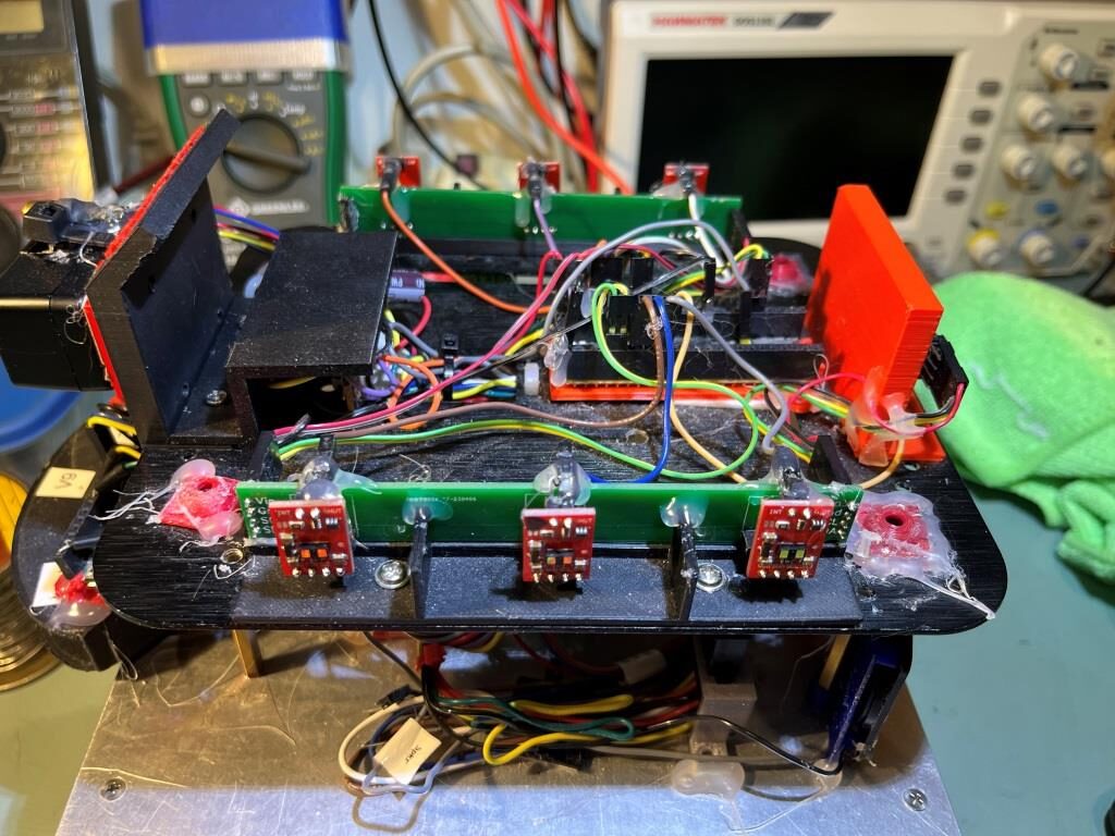
The next step was to load ‘WallE3_Complete_V2.ino’ onto the Teensy 3.5 main controller and verify that it could indeed get distance information from the second-deck Teensy 3.5 VL53L1X array controller. Here’s some output from WallE3_Complete_V2.ino in ‘DISTANCES_ONLY’ mode. Again I used my hand to block the left, right, and rear sensors to verify proper operation.
|
1 2 3 4 5 6 7 8 9 10 11 12 13 14 15 16 17 18 19 20 21 22 23 24 25 26 27 28 29 30 31 32 33 34 35 36 37 38 39 40 41 42 43 44 45 46 47 48 49 50 51 52 53 54 55 56 57 58 59 60 61 62 63 64 65 66 67 68 69 70 71 72 73 74 75 76 77 78 79 80 81 82 83 84 85 86 87 88 89 90 91 92 93 94 95 96 97 98 99 100 101 102 103 104 105 106 107 108 109 110 111 112 113 114 115 116 117 118 119 120 121 122 123 124 125 126 127 128 129 130 131 132 133 134 135 136 137 138 |
Opening port Port open gl_pSerPort now points to active Serial (USB or Wixel) 7950: Starting setup() for WallE3_Complete_V2.ino Checking for MPU6050 IMU at I2C Addr 0x68 MPU6050 connection successful Initializing DMP... Enabling DMP... DMP ready! Waiting for MPU6050 drift rate to settle... Calibrating...Retrieving Calibration Values Msec Hdg 10581 -0.059 -0.045 MPU6050 Ready at 10.58 Sec with delta = -0.014 Checking for Teensy 3.5 VL53L0X Controller at I2C addr 0x20 Teensy available at 11681 with gl_bVL53L0X_TeensyReady = 1. Waiting for Teensy setup() to finish 11684: got 1 from VL53L0X Teensy Teensy setup() finished at 11787 mSec VL53L0X Teensy Ready at 11789 Checking for Garmin LIDAR at Wire2 I2C addr 0x62 LIDAR Responded to query at Wire2 address 0x62! Setting LIDAR acquisition repeat value to 0x02 for <100mSec measurement repeat delay Initializing Front Distance Array...Done Initializing Rear Distance Array...Done ------------ DISTANCES ONLY MODE!!! ----------------- Msec LFront LCenter LRear RFront RCenter RRear Rear LSteer RSteer LIDAR 11837 26.00 21.00 21.00 200.00 200.00 63.00 137.00 79 0.51 1.00 11911 26.00 20.00 21.00 200.00 200.00 63.00 137.00 78 0.52 1.00 12011 26.00 20.00 21.00 200.00 200.00 66.00 137.00 81 0.50 1.00 12111 26.00 21.00 21.00 200.00 200.00 64.00 137.00 82 0.52 1.00 12211 26.00 21.00 21.00 200.00 200.00 63.00 137.00 82 0.50 1.00 12311 26.00 21.00 21.00 200.00 200.00 65.00 137.00 83 0.52 1.00 12411 26.00 21.00 21.00 200.00 200.00 65.00 137.00 82 0.49 1.00 12511 26.00 21.00 21.00 200.00 200.00 64.00 137.00 82 0.51 1.00 12611 26.00 21.00 21.00 200.00 200.00 63.00 138.00 81 0.50 1.00 12711 26.00 21.00 21.00 200.00 200.00 65.00 138.00 83 0.48 1.00 12811 26.00 21.00 21.00 200.00 200.00 65.00 138.00 81 0.55 1.00 12911 26.00 21.00 21.00 200.00 200.00 66.00 138.00 82 0.53 1.00 13011 27.00 21.00 21.00 200.00 200.00 61.00 137.00 81 0.57 1.00 13111 26.00 21.00 21.00 200.00 200.00 58.00 137.00 81 0.52 1.00 13211 26.00 20.00 21.00 200.00 5.00 0.00 137.00 81 0.52 1.00 13310 26.00 21.00 21.00 0.00 0.00 0.00 137.00 82 0.51 0.00 13411 26.00 20.00 21.00 1.00 0.00 0.00 137.00 81 0.48 0.10 13511 26.00 20.00 21.00 0.00 0.00 0.00 138.00 81 0.50 0.00 13611 26.00 20.00 21.00 0.00 0.00 0.00 138.00 81 0.51 0.00 Msec LFront LCenter LRear RFront RCenter RRear Rear Front LSteer RSteer 13711 26.00 20.00 21.00 0.00 0.00 0.00 137.00 81 0.52 0.00 13811 27.00 21.00 21.00 0.00 0.00 0.00 138.00 83 0.55 0.00 13911 26.00 21.00 21.00 0.00 0.00 0.00 138.00 81 0.51 0.00 14011 26.00 21.00 21.00 0.00 0.00 0.00 137.00 81 0.50 0.00 14111 27.00 21.00 21.00 0.00 0.00 0.00 138.00 82 0.56 0.03 14211 26.00 21.00 21.00 3.00 0.00 0.00 138.00 81 0.51 0.32 14311 26.00 20.00 21.00 2.00 0.00 0.00 137.00 82 0.51 0.22 14411 26.00 21.00 21.00 0.00 0.00 0.00 138.00 80 0.48 0.09 14511 26.00 21.00 21.00 200.00 0.00 0.00 138.00 81 0.56 0.00 14611 26.00 21.00 21.00 200.00 200.00 0.00 137.00 81 0.53 1.00 14711 26.00 21.00 21.00 200.00 200.00 0.00 137.00 81 0.53 1.00 14811 26.00 21.00 21.00 200.00 200.00 16.00 137.00 82 0.50 1.00 14911 26.00 20.00 21.00 200.00 200.00 12.00 138.00 83 0.53 1.00 15011 26.00 21.00 21.00 200.00 200.00 13.00 138.00 81 0.49 1.00 15111 26.00 21.00 21.00 200.00 200.00 18.00 137.00 82 0.52 1.00 15211 26.00 21.00 21.00 200.00 200.00 66.00 137.00 82 0.53 1.00 15311 26.00 21.00 21.00 200.00 200.00 107.00 137.00 83 0.58 1.00 15411 26.00 20.00 21.00 200.00 200.00 95.00 138.00 82 0.50 1.00 15511 1.00 21.00 21.00 200.00 200.00 189.00 137.00 81 -1.00 1.00 15611 0.00 0.00 11.00 200.00 200.00 200.00 138.00 81 -1.00 0.21 Msec LFront LCenter LRear RFront RCenter RRear Rear Front LSteer RSteer 15711 0.00 0.00 1.00 200.00 200.00 200.00 137.00 81 -0.11 1.00 15811 0.00 0.00 1.00 200.00 200.00 200.00 138.00 81 -0.11 1.00 15911 0.00 0.00 1.00 200.00 200.00 200.00 138.00 83 -0.12 1.00 16011 0.00 0.00 0.00 200.00 200.00 186.00 137.00 81 -0.06 1.00 16111 0.00 0.00 1.00 200.00 200.00 200.00 137.00 82 -0.05 1.00 16211 0.00 0.00 4.00 200.00 200.00 200.00 137.00 82 -0.47 -0.57 16311 5.00 20.00 22.00 200.00 200.00 200.00 137.00 81 -1.00 0.45 16411 1.00 20.00 22.00 200.00 194.00 200.00 137.00 82 -1.00 1.00 16511 4.00 20.00 23.00 200.00 200.00 200.00 138.00 81 -1.00 1.00 16611 4.00 21.00 23.00 200.00 200.00 200.00 137.00 81 -1.00 1.00 16711 4.00 20.00 7.00 200.00 200.00 184.00 138.00 81 -0.36 1.00 16811 4.00 9.00 3.00 200.00 200.00 200.00 138.00 81 0.08 1.00 16911 2.00 0.00 3.00 200.00 200.00 200.00 137.00 81 -0.02 1.00 17011 1.00 0.00 1.00 200.00 200.00 200.00 138.00 81 0.06 1.00 17110 1.00 0.00 1.00 200.00 200.00 200.00 137.00 82 0.07 1.00 17211 0.00 0.00 0.00 200.00 200.00 200.00 137.00 83 -0.09 -0.24 17311 0.00 0.00 1.00 200.00 200.00 200.00 137.00 83 -0.10 -1.00 17411 4.00 6.00 16.00 200.00 200.00 200.00 137.00 83 -1.00 1.00 17511 9.00 13.00 22.00 200.00 200.00 23.00 137.00 83 -1.00 1.00 17611 27.00 20.00 23.00 200.00 13.00 3.00 138.00 82 0.37 1.00 Msec LFront LCenter LRear RFront RCenter RRear Rear Front LSteer RSteer 17711 27.00 20.00 22.00 200.00 16.00 6.00 138.00 81 0.47 1.00 17811 26.00 21.00 22.00 200.00 200.00 10.00 138.00 81 0.43 1.00 17911 26.00 21.00 23.00 200.00 200.00 32.00 137.00 82 0.27 1.00 18011 26.00 20.00 23.00 200.00 200.00 36.00 137.00 82 0.28 1.00 18111 26.00 20.00 22.00 200.00 200.00 38.00 137.00 82 0.40 1.00 18211 26.00 20.00 22.00 200.00 200.00 36.00 138.00 81 0.45 1.00 18311 26.00 21.00 22.00 200.00 200.00 33.00 0.00 80 0.44 1.00 18411 26.00 20.00 22.00 200.00 200.00 29.00 0.00 80 0.44 1.00 18511 26.00 20.00 22.00 200.00 200.00 24.00 0.00 81 0.41 1.00 18611 27.00 21.00 22.00 200.00 200.00 25.00 0.00 81 0.46 1.00 18711 26.00 21.00 22.00 200.00 200.00 31.00 0.00 80 0.40 1.00 18811 26.00 21.00 23.00 200.00 200.00 33.00 0.00 82 0.36 1.00 18911 26.00 21.00 22.00 200.00 200.00 39.00 0.00 82 0.40 1.00 19011 27.00 21.00 22.00 200.00 200.00 41.00 149.00 81 0.48 1.00 19111 26.00 21.00 23.00 200.00 128.00 40.00 138.00 82 0.35 1.00 19211 27.00 20.00 22.00 200.00 200.00 42.00 138.00 81 0.42 1.00 19311 26.00 21.00 23.00 200.00 200.00 44.00 137.00 81 0.35 1.00 19410 27.00 21.00 22.00 200.00 200.00 49.00 138.00 80 0.42 1.00 19511 27.00 21.00 22.00 200.00 200.00 64.00 138.00 82 0.42 1.00 19611 26.00 21.00 22.00 200.00 200.00 65.00 138.00 81 0.48 1.00 Msec LFront LCenter LRear RFront RCenter RRear Rear Front LSteer RSteer 19711 26.00 21.00 22.00 200.00 200.00 70.00 138.00 80 0.37 1.00 19811 26.00 21.00 22.00 200.00 200.00 68.00 138.00 81 0.39 1.00 19911 27.00 21.00 22.00 200.00 200.00 65.00 138.00 83 0.48 1.00 20011 26.00 20.00 22.00 200.00 200.00 69.00 138.00 81 0.44 1.00 20111 26.00 20.00 22.00 200.00 200.00 73.00 137.00 82 0.42 1.00 20211 26.00 21.00 23.00 200.00 200.00 69.00 137.00 82 0.35 1.00 20311 27.00 21.00 22.00 200.00 200.00 67.00 137.00 82 0.45 1.00 20411 27.00 21.00 22.00 200.00 200.00 71.00 137.00 82 0.46 1.00 20511 26.00 21.00 22.00 200.00 200.00 72.00 138.00 82 0.42 1.00 20611 27.00 21.00 22.00 200.00 200.00 67.00 138.00 82 0.48 1.00 20711 27.00 21.00 22.00 200.00 200.00 70.00 138.00 81 0.45 1.00 20811 26.00 21.00 22.00 200.00 200.00 68.00 138.00 81 0.40 1.00 20911 26.00 21.00 22.00 200.00 200.00 71.00 138.00 80 0.42 1.00 21011 26.00 21.00 23.00 200.00 200.00 70.00 137.00 80 0.37 1.00 21111 26.00 21.00 22.00 200.00 200.00 66.00 138.00 82 0.42 1.00 21211 26.00 21.00 22.00 200.00 200.00 70.00 137.00 83 0.41 1.00 21311 26.00 21.00 22.00 200.00 200.00 70.00 138.00 82 0.46 1.00 Port closed |
The next step is to re-implement the distance compensation algorithms for each sensor. For the VL53L0X sensors, this was done using the procedure described in this post. The procedure involves taking sensor readings at several known distances, and using the data to develop a correction expression for each sensor.
To make this happen, I had to first disable the current compensation scheme for all the sensors. Then I ran ‘WallE3_Complete_V2.ino’ again in Distances Only mode to get the data needed to develop the compensation expressions.
Stay tuned,
Frank