Posted 06/18/16
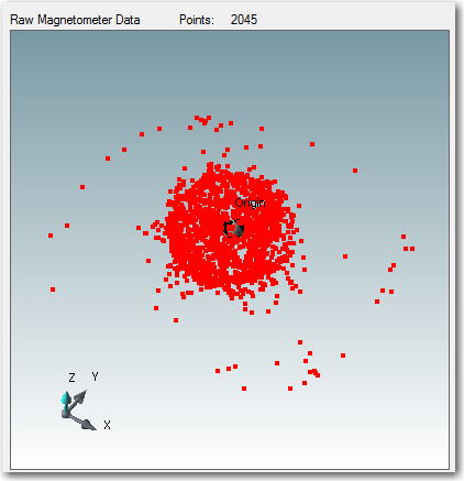
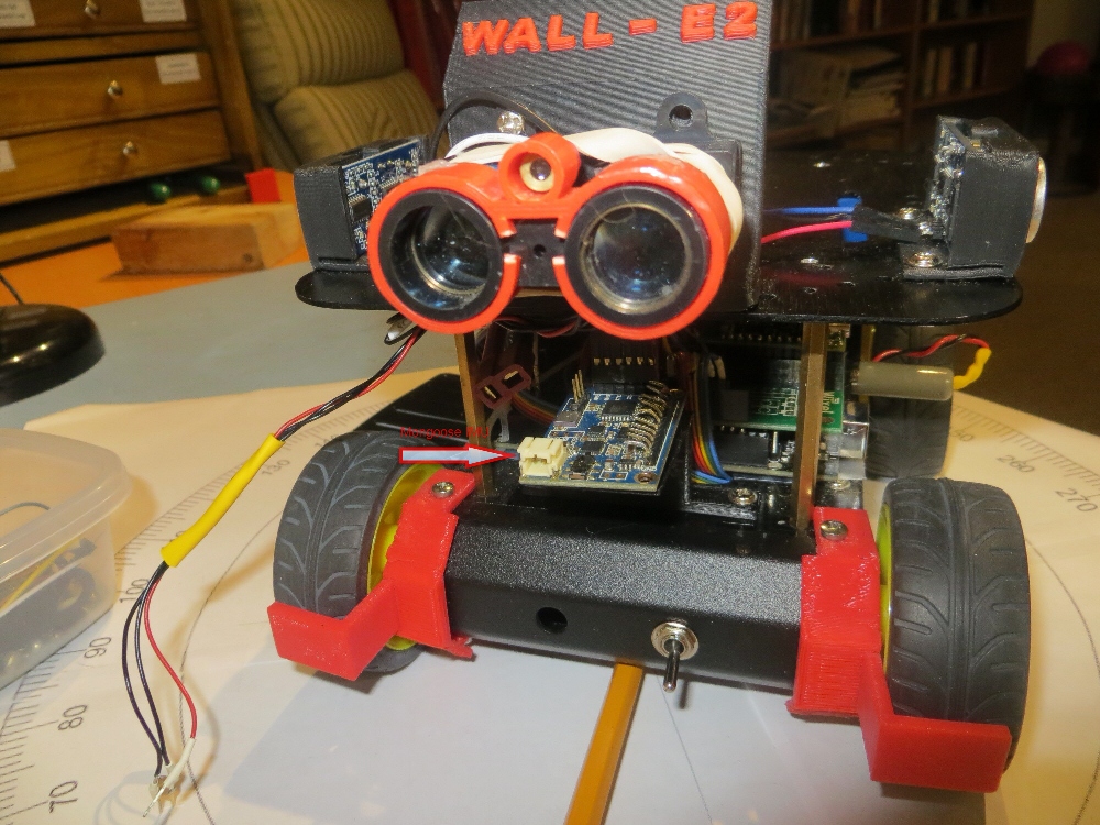
My last few posts have described my efforts to create an easy-to-use magnetometer calibration utility to allow for as-installed magnetometer calibration. In situ calibration is necessary for magnetometers because they can be significantly affected by nearby ‘hard’ and ‘soft’ iron interferers. In my research on this topic, I discovered there were two main magnetometer calibration methods; in one, 3-axis magnetometer data is acquired with the entire assembly containing the magnetometer placed in a small but complete number of well-known positions. The data is then manipulated to generate calibration values that are then used to convert magnetometer data at an arbitrary position. The other method involves acquiring a large amount (hundreds or thousands of points) of data while the assembly is rotated arbitrarily around all three axes. The compensation method assumes the acquired data is sufficiently varied to cover the entire 3D sphere, and then finds the best fit of the data to a perfect sphere centered at the origin. This produces an upper triangular 3×3 matrix of multiplicative values and an offset vector that can be used to convert any magnetometer position raw value to a compensated one. I decided to create a tool using the second method, mainly because I had available a MATLAB script that would do most of the work for me, and Octave, the free open-source application that can execute most MATLAB scripts. Moreover, Octave for windows can be called from C#/.NET programs, making it a natural fit for my needs. In any case, I was able to implement the utility (twice!!) over the course of a couple of months, getting it to the point where I am now ready to try calibrating my CK Devices ‘Mongoose’ IMU, as installed on my ‘Wall-E2’ four-wheel drive robot.
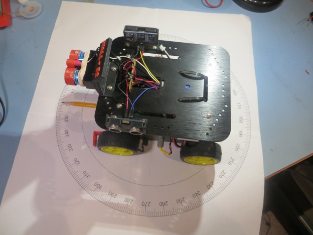
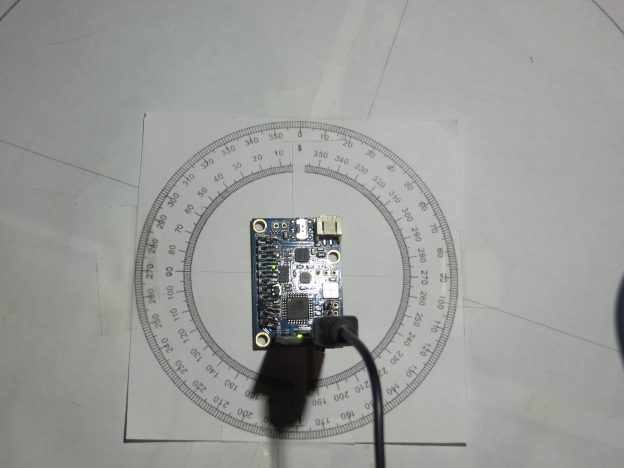
However, before mounting the IMU on the robot and going for ‘the big Kahuna’ result, I decided to essentially re-create my original experiment with the IMU rotated in the X-Y plane on my bench-top, as described in the post ‘Giving Wall-E2 A Sense of Direction – Part III‘. My 4-inch compass rose had long since bitten the dust, but I had saved the print file (did I tell you that I never throw anything away)
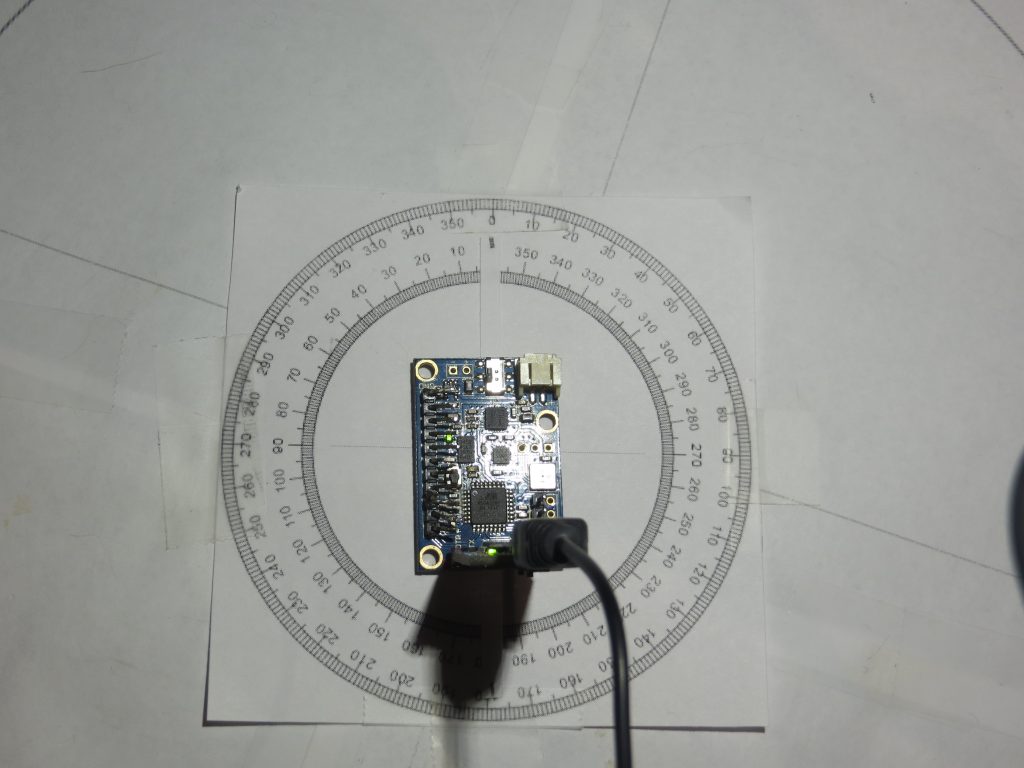
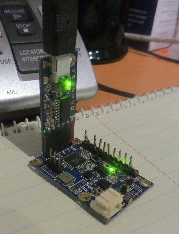
Mongoose IMU on 4-Inch Compass Rose
So, I basically re-created the original heading error test from back in March, and got similar (but not identical) results, as shown below:
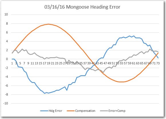
Heading Error, Compensation, and Comp+Error
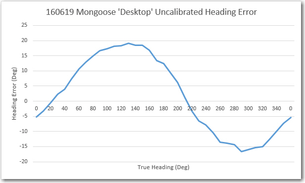
06/19/16 Mongoose ‘Desktop’ Heading Error
Then I used my newly minted magnetometer calibration utility to generate a calibration matrix and center offset, so I can apply them to the above data. However, before I can do that I have to go back into CK Devices original code to find out where the calibration should be applied – more digging :-(.
In the original Mongoose IMU code, the function ‘ReadCompass()’ in HMC5883L.ino gets the raw values from the magnetometer and generates compensated values using whatever values the user places in two ‘struct’ objects (all zeros by default). However, I was clever enough to only send the ‘raw’ uncalibrated magnetometer data to the serial port, so that is what I’ve been using as ‘raw’ data for my mag calibration tool – so far, so good. However, what I need for my robot is compensated values, so (hopefully) I can (accurately?) determine Wall-E2’s heading.
So, it appears I have two options here; I can continue to emit ‘raw’ data from the Mongoose and perform any needed compensation externally, or I can do the compensation internally to the Mongoose and emit only corrected mag data. The problem with the latter option (internal to the Mongoose) is that I would have to defeat it each time the robot configuration changed, with it’s inevitable change to the magnetometer’s surroundings. If I write an external routine to do the compensation based on the results from the calibration tool, then it is only that one routine that will require an update. OTOH, If the compensation is internal to the Mongoose, then modularity is maximized – a very good feature. The deciding factor is that if the routine is internal to the Moongoose, then I can remove it from the robot and I still have a complete setup for magnetometer work. So, I decided to write it into the Mongoose code, but have the ability to switch it in/out with a compile time switch (something like NO_MAGCOMP?)
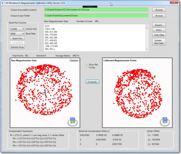
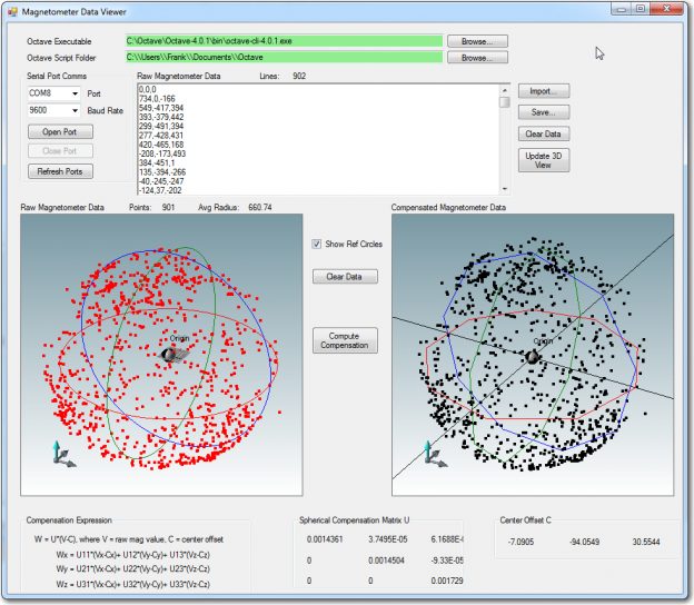
The compensation expression being implemented is:
W = U*(V-C), where U = spherical compensation matrix, V = raw mag values, C = center offset value
Since U is always upper triangular (don’t ask – I don’t know why), the above matrix expression simplifies to:
Wx = U11*(Vx-Cx) + U12*(Vy-Cy) + U13*(Vz-Cz)
Wy = U22*(Vy-Cy) + U23*(Vz-Cz)
Wz = U33*(Vz-Cz)
I implemented the above expression in the Mongoose firmware by adding a new function ‘CalibrateMagData()’ as follows:
|
1 2 3 4 5 6 7 8 9 10 11 12 13 14 15 16 17 18 19 20 21 22 |
void CalibrateMagData() { //Purpose: Apply spherical compensation expression (vals from mag cal tool) //Expression is W = U*(V-C), where U is u.t. comp matrix, V is raw data, C is ctr offset float raw_x = sen_data.magnetom_x_raw; float raw_y = sen_data.magnetom_y_raw; float raw_z = sen_data.magnetom_z_raw; //X-component sen_data.magnetom_x = magcalvals.U11*(raw_x - magcalvals.Cx) + magcalvals.U12*(raw_y - magcalvals.Cy) + magcalvals.U13*(raw_z - magcalvals.Cz); //Y-component sen_data.magnetom_y = magcalvals.U22*(raw_y - magcalvals.Cy) + magcalvals.U23*(raw_z - magcalvals.Cz); //Z-component sen_data.magnetom_z = magcalvals.U33*(raw_z - magcalvals.Cz); } |
Using the already existing s_sensor_data struct which is defined as follows:
|
1 2 3 4 5 6 7 8 9 10 11 12 13 14 15 16 17 18 19 20 21 22 23 24 25 26 27 28 |
struct s_sensor_data { //raw data is uncorrected and corresponds to the //true sensor axis, not the redefined platform orientation int gyro_x_raw; int gyro_y_raw; int gyro_z_raw; int accel_x_raw; int accel_y_raw; int accel_z_raw; int magnetom_x_raw; int magnetom_y_raw; int magnetom_z_raw; //This data has been corrected based on the calibration values float gyro_x; float gyro_y; float gyro_z; float accel_x; float accel_y; float accel_z; float magnetom_x; float magnetom_y; float magnetom_z; float magnetom_heading; short baro_temp; long baro_pres; }; |
Then I created another ‘print’ routine, ‘PrintMagCalData()’ to print out the calibrated (vs raw) magnetometer data. Also, after an overnight dream-state ‘aha’ moment, I realized I don’t have to incorporate a compile-time #ifdef statement to switch between ‘raw’ and ‘calibrated’ data readout from the Mongoose – I simply attach a jumper from either GND or +3.3V to one of the I/O pins, and implement code that calls either ‘PrintMagCalData()’ or ‘PrintMagRawData()’ depending on the HIGH/LOW state of the monitor pin. Now that’s elegant! 😉
After making these changes, I fired up just the Mongoose using VS2015 in debug mode, which includes a port monitor function. As soon as the Moongoose came up, it started spitting out 3D magnetometer data – YAY!!
It’s been a few days since I got this going – my wife and I went off to a weekend bridge tournament in Kentucky and we got back late last night – so I didn’t get a chance to compare the ‘after-calibration’ heading performance with the ‘before’ version until today.
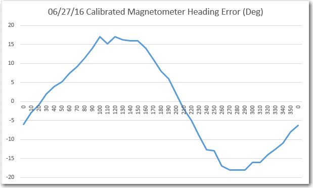
After Calibration Magnetic Heading Error
Comparing the above chart to the one from 6/19, it is clear that they are virtually identical. I guess what this means is that, at least for the ‘free space’ case with no nearby interferers, calibration doesn’t do much. Also, this implies that the heading errors observed above have nothing to do with external influences – they are ‘baked in’ to the magnetometer itself. The good news is, a sine function correction table should take most of this error out, assuming more accurate heading measurements are required (I don’t ).
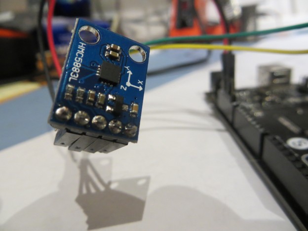
In summary, at this point I have a working magnetometer calibration tool, and I have used it successfully to generate calibration matrix/center offset values for my Mongoose IMU’s HMC5883 magnetometer component. After calibration, the ‘free space’ heading performance is essentially unchanged, as there were no significant ‘hard’ or ‘soft’ iron interferers to calibrate out.
Next up – remount the Mongoose on my 4WD robot, where there are plenty of hard/soft iron interference sources, and see whether or not calibration is useful.