Posted 30 April 2019
In two previous posts (here & here) I described my efforts to upgrade Wall-E2’s wall following performance using a PID control algorithm. The results of my efforts to date in this area have not been very spectacular – a better description might actually be ‘dreadful’ :-(.
After some additional analysis, I came to believe that the reason the PID approach doesn’t work very well is a fundamental feature of the way Wall-E2 measures distance to the nearest wall. Wall-E2 has two acoustic sonar units fixed to its upper deck, and they measure the distance perpendicular to the robot’s longitudinal axis. What this means, however, is that when the robot is angled with respect to the nearest wall, the distance measured isn’t the perpendicular distance, but rather the hypotenuse of the right triangle with the right angle at the wall. So, when Wall-E2 turns toward or away from the wall, the measured distance increases even though the robot hasn’t actually moved toward or away. Conversely, if the robot is angled in toward the wall and then turns to be parallel, the measured distance decreases even if the robot hasn’t moved at all relative to that wall. The situation is shown in the sketch below:
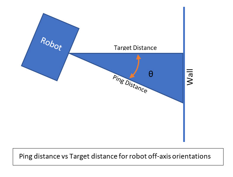
Using Excel, I ran a simulation of the ping distance versus the actual distance for a range of angle offsets from 0 to 30 degrees, as shown below:
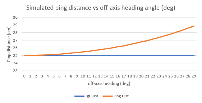
As shown above, the ping distance for a constant 25 cm offset ranges from 25 (robot longitudinal axis parallel to the wall) to almost 29 cm for a 30 degree off-axis heading. These values translate to a percentage error of zero to approximately 15%, independent of the initial parallel distance.
So, it becomes obvious why a standard PID algorithm has trouble; if the ping distance goes up slightly, the PID algorithm attempts to compensate by turning toward the wall. However, this causes the ping distance to increase rather than decrease, causing the algorithm to command an even greater angle toward the wall, which in turn causes a further increase in ping distance – entirely backward. The reverse happens for an initial decrease in the ping distance starting from a parallel orientation. The algorithm commands a turn away from the wall, which causes the ping distance to increase immediately, even though the actual distance hasn’t changed. This causes the algorithm to seriously overcorrect in one case, and seriously undercorrect in the other. Not good.
What I need is a way to compensate for the changes in ping distance caused by Wall-E2’s angular orientation with respect to the wall being tracked. If Wall-E2 is oriented parallel to the wall, then no correction is needed; if not,then a correction is required. Fortunately for the good guys, Wall-E2 now has a way of providing the needed heading information, with the integration of the MPU6050-based 6DOF IMU module described in this post from last September.
To investigate this idea, I modified an old test program to have Wall-E2 perform a series of mild S-turns in my test hallway while capturing heading and ping distance data. The S-turns were tweaked so that Wall-E2 stayed a fairly constant 50 cm from the right-hand wall, as shown in the following movie clip.
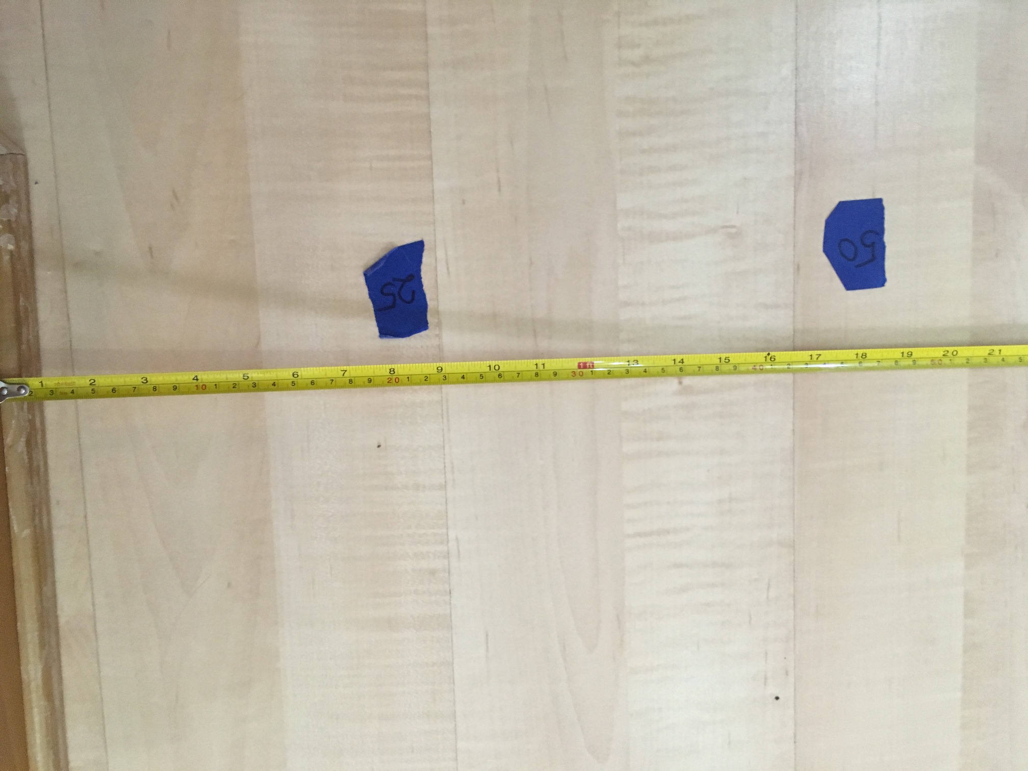
Start of test area showing tape measure for offset distance measurement
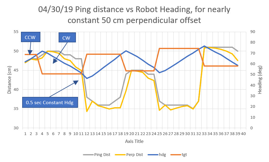
Using Excel, I plotted the reported ping distance, the commanded heading, and the actual heading versus time, as shown below:
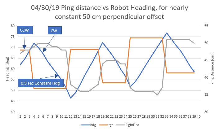
In the above plot, the initial CCW turn (away from the wall) was a 10° change, and all the rest were approximately 20° to maintain a more-or-less straight line. At the end of the second (the first CW turn) and subsequent heading changes, there is an approximately 0.5 sec straight period, during which no data was captured. As can be seen, the ping distance (gray curve) goes up slightly as the first CCW turn starts, then levels off during the changeover from CCW to CW turns, and then precipitously declines as the CW turn sweeps the ping sensor toward the perpendicular point. Part of this decline is actual distance change caused by the 0.5 sec straight period that moves the robot toward the wall. After the next (CCW) heading change is commanded, the robot starts to turn away from the wall causing the ping distance to increase, but this is partially cancelled by the fact that the robot continues to travel toward the wall during the S-turn. As soon as the robot gets parallel to the wall, then the ping distance goes up quickly as the heading continues to change in a CCW direction. This behavior repeats for each S-turn until the end of the run.
As an exercise, I added another column to the spreadsheet – “perpendicular distance”, and set up a formula to compute the adjusted distance from the robot to the wall, using the recorded angular offset. This computation presumes that the robot started off parallel to the wall (confirmed via the video clip). The result is shown on the yellow line in the plot below:
Ping distance and heading vs time, with calculated perpendicular distance added
As can be seen from the above plot and video, the compensated distance looks like it might be a good match with the perpendicular distance estimated from the video. For instance, at 17 sec into the video, the robot has just finished the first clockwise turn and straight run, and is just starting the second counter-clockwise turn. At this point the robot is oriented parallel to the wall, and the ping distance and the perpendicular distance should match. The video shows that distance should be about 33-35 cm, and the recorded ping distance at this point is 36 cm. However, the calculated distance went directly from 45 cm at point 11 to 34 cm at point 12 and basically stayed at that value before changing rapidly from 34 to 45 over points 19 & 20. Again at 19 seconds into the video, the robot is approximately 42-44 cm from the wall and parallel to it; both the actual ping distance and the calculated perpendicular distance agree at this point at 45 cm – a close match to the estimate from the video.
So now the question is – can I use the calculated perpendicular wall distance to assist wall-following operations? A significant issue may be knowing when the robot is actually parallel to the wall, to establish a heading baseline for compensation calcs.
When is the robot parallel to the wall?
A unique feature of the point or points where the robot is parallel to the wall is that the ping distance and the calculated distance are equal. However, that’s a bit of ‘chicken and the egg’ as one has to know the robot is parallel in order to use an offset angle of 0 degrees for the compensation calc to work out. Since the heading information available from the MPU6050 IMU is only relative, the heading value for the parallel condition can be anything, and can vary arbitrarily from run to run. So, what to do? One thought would be to have the robot make a short S-turn at the start of any tracking run to establish the heading for which the ping distance goes through a minimum or maximum – the heading for the max/min point would be the parallel heading. From there on, that heading should be reliably constant until the next time the robot’s power is cycled. Of course, a new parallel heading value would be required each and every time Wall-E2’s tracking situation changes (obstacle recovery, step-turns and reversals at the end of a hallway, changing from the left wall to the right one, etc). Maybe a hybrid mode would be feasible, whereby the robot uses uncompensated heading-based S-turns instead of the current ‘bang-bang’ system for initial wall tracking, shifting to a compensation algorithm after a suitable parallel heading is determined.
Looking at the above plots, it may not be all that useful to look for maxima and/or minima, as there are multiple headings for which the ping distance is constant, so which one is the parallel heading? Thinking about ways to rapidly find the parallel heading, it occurred to me that my previous work on quickly finding the mathematical variance of a set of values might be useful here. I plugged the above ping distance numbers into the Excel spreadsheet I used before, and got the following plot of ping distance and 3-element running variance vs time.
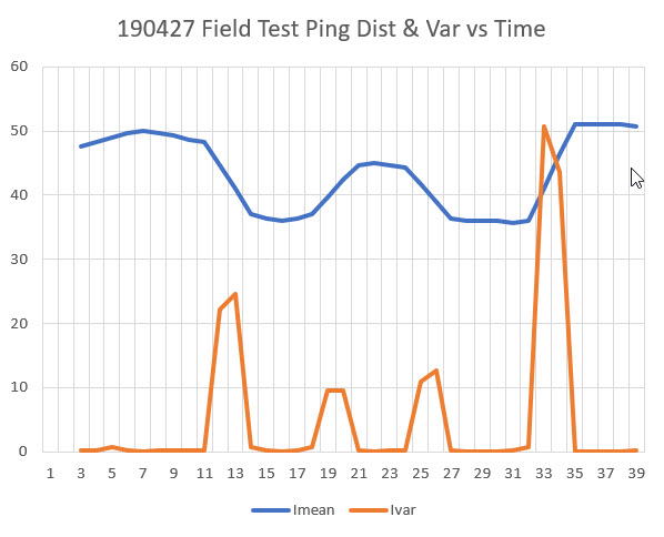
So, looking at the above plot, it is encouraging that a 3-point running variance calculation shows near-zero values when the robot is most probably parallel or nearly parallel to the wall. Adding the heading information to the spreadsheet gives the plot shown below
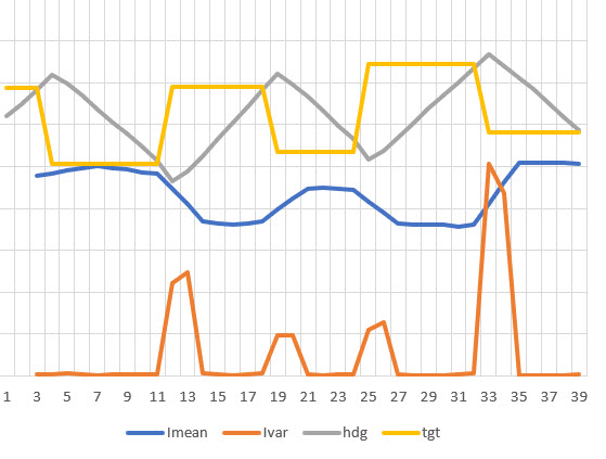
and now it is clear that the large variance values are associated with the changes from one heading to another, and the low variance values are associated with the middle section of each linear heading change (S-turn) segment. If I further enhance the plot by putting the variance plot on a secondary scale and zooming in on the low variance sections, we get the plot shown below:
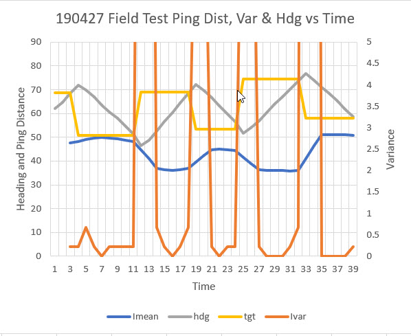
Variance scale modified to show 0-5 range only
In the above plot, the variance line is zoomed in to the 0-5 range only, emphasizing the 0-0.5 unit variance range. In this plot it can be seen that the variance actually has a distinct minimum very near zero at time points 7, 16, 22, 28-30, and 35-38. These time values correspond to robot heading values of 64, 61, 63, 61-67. and 70-65. Discarding the last set as bad data (this is where the robot literally ‘hit the wall’ at the end of the run), we can compute an approximate parallel heading value as the average of all these values, or the average of 64, 61, 63, 64 (average of 61-67) = 63 degrees. From the video we can see that the robot started out parallel to the wall, and the first heading reading was 62 degrees – a very good match to the calculated parallel heading value.
The next step, I think, is to run some more field tests against a wall, with wall-following and heading assist integrated into the code.
Frank