Teensy | Paynter's Palace

Posted 18 June 2017

In my last post on this subject, I showed how I could speed up ADC cycles for the Teensy 3.5 SBC, ending up with a configuration that took only about 5Î¼Sec/analog read. This in turn gave me some confidence that I could implement a full four-sensor digital BPF running at 20 samples/cycle at 520Hz without running out of time.

So, I decided to code this up in an Arduino sketch and see if my confidence was warranted. The general algorithm for one sensor channel is as follows:

Collect a 1/4 cycle group of samples, and add them all to form a ‘sample_group’
For each sample_group, form I & Q components by multiplying the single sample_group by the appropriate sign for that position in the cycle. The sign sequence for I is (+,+,-,-), and for Q it is (-,+,+,-) .
Perform steps 1 & 2 above 4 times to collect an entire cycle’s worth of samples. As each I/Q sample_group component is generated, add it to a ‘cycle_group_sum’ – one for the I and one for the Q component.
When a new set of cycle_group_sums (one for I, one for Q) is completed, use it to update a set of two N-element running sums (one for I, one for Q).
Add the absolute values of the I & Q running sums to form the final demodulated signal value for the sensor channel.

To generalize the above algorithm for K sensor channels, the ‘sample_group’ and ‘cycle_group_sum’ variables become K-element arrays, and each step becomes a K-step loop. The N-element running sum arrays (circular buffers) become [K][M] arrays, i.e. two M-element array for each sensor (one for I, one for Q).

All of the above sampling, summing, and circular buffer management must take place within the ~96μSec ‘window’ between samples, but not all steps have to be performed each time. A new sample for each sensor channel is acquired at each point, but sample groups are converted to cycle group sums only once every 5 passes, and the running sum and final values are only updated every 20 passes.

I built up the algorithm in VS2017 and put in some print statements to show how the gears are turning. In addition, I added code to set a digital output HIGH at the start of each sample window, and LOW when all processing for that pass was finished. The idea is that if the HIGH portion of the pulse is less than the available window time, all is well. When I ran this code on my Teensy 3.5, I got the following print output (truncated for brevity)

RunningSumInsertionIndex = 63
SampleSumCount = 0
SampleSumCount = 1
SampleSumCount = 2
SampleSumCount = 3
SampleSumCount = 4
CycleGroupSumCount = 0
SampleSumCount = 0
SampleSumCount = 1
SampleSumCount = 2
SampleSumCount = 3
SampleSumCount = 4
CycleGroupSumCount = 1
SampleSumCount = 0
SampleSumCount = 1
SampleSumCount = 2
SampleSumCount = 3
SampleSumCount = 4
CycleGroupSumCount = 2
SampleSumCount = 0
SampleSumCount = 1
SampleSumCount = 2
SampleSumCount = 3
SampleSumCount = 4
CycleGroupSumCount = 3
RunningSumInsertionIndex = 0
SampleSumCount = 0
SampleSumCount = 1
SampleSumCount = 2
SampleSumCount = 3
SampleSumCount = 4
CycleGroupSumCount = 0
SampleSumCount = 0
SampleSumCount = 1
SampleSumCount = 2
SampleSumCount = 3
SampleSumCount = 4
CycleGroupSumCount = 1
SampleSumCount = 0
SampleSumCount = 1
SampleSumCount = 2
SampleSumCount = 3
SampleSumCount = 4
CycleGroupSumCount = 2
SampleSumCount = 0
SampleSumCount = 1
SampleSumCount = 2
SampleSumCount = 3
SampleSumCount = 4
CycleGroupSumCount = 3
RunningSumInsertionIndex = 1
SampleSumCount = 0
SampleSumCount = 1

RunningSumInsertionIndex = 63

SampleSumCount = 0

SampleSumCount = 1

SampleSumCount = 2

SampleSumCount = 3

SampleSumCount = 4

CycleGroupSumCount = 0

SampleSumCount = 0

SampleSumCount = 1

SampleSumCount = 2

SampleSumCount = 3

SampleSumCount = 4

CycleGroupSumCount = 1

SampleSumCount = 0

SampleSumCount = 1

SampleSumCount = 2

SampleSumCount = 3

SampleSumCount = 4

CycleGroupSumCount = 2

SampleSumCount = 0

SampleSumCount = 1

SampleSumCount = 2

SampleSumCount = 3

SampleSumCount = 4

CycleGroupSumCount = 3

RunningSumInsertionIndex = 0

SampleSumCount = 0

SampleSumCount = 1

SampleSumCount = 2

SampleSumCount = 3

SampleSumCount = 4

CycleGroupSumCount = 0

SampleSumCount = 0

SampleSumCount = 1

SampleSumCount = 2

SampleSumCount = 3

SampleSumCount = 4

CycleGroupSumCount = 1

SampleSumCount = 0

SampleSumCount = 1

SampleSumCount = 2

SampleSumCount = 3

SampleSumCount = 4

CycleGroupSumCount = 2

SampleSumCount = 0

SampleSumCount = 1

SampleSumCount = 2

SampleSumCount = 3

SampleSumCount = 4

CycleGroupSumCount = 3

RunningSumInsertionIndex = 1

SampleSumCount = 0

SampleSumCount = 1

And the digital output pulse on the scope is shown in the following photo

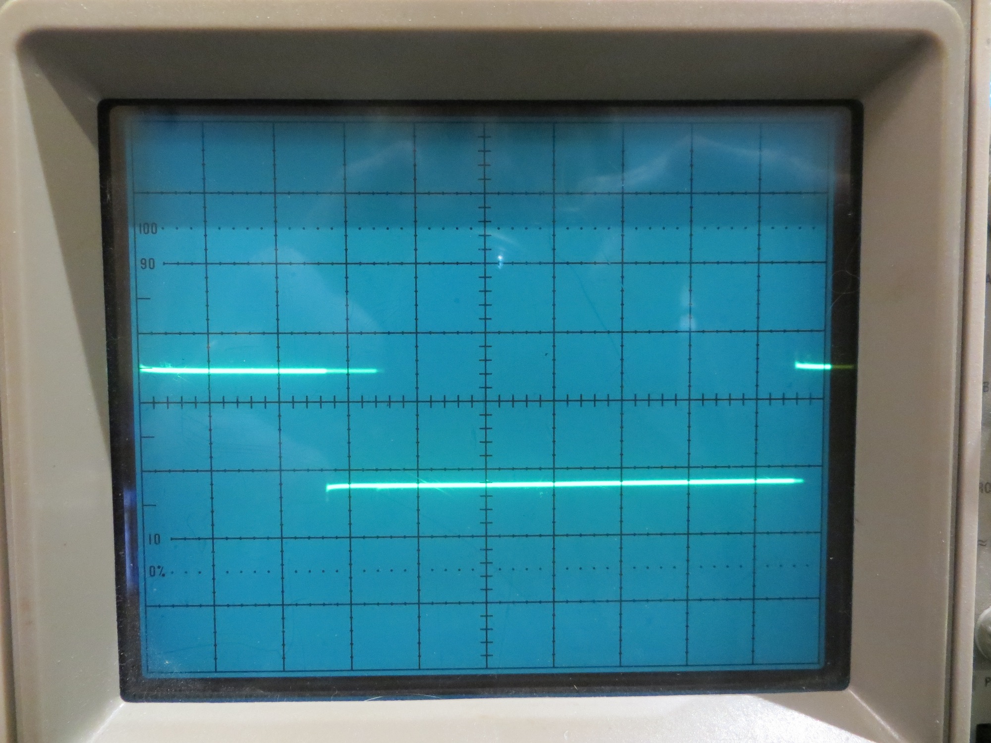
Timing pulse for BPF algorithm run, shown at 10uS/cm. Note the time between rising edges is almost exactly 96uSec, and there is well over 60uSec ‘free time’ between the end of processing and the start of the next acquisition window.

As can be seen in the above photo, there appears to be plenty of time (over 60μSec) remaining between the end of processing for one acquisition cycle, and the start of the next acquisition window. Also, note the fainter ‘fill-in’ section over the LOW part of the digital output. I believe this shows that not all acquisition cycles take the same amount of processing time. Four acquisition cycles out of every 5 require much less processing, as all that happens is the individual samples are grouped into a ‘sample_group’. So the faint ‘fill-in’ section probably shows the additional time required for the processing that occurs after collection/summation of each ‘sample_group’.

The code for these measurements is included below:

//Program to implement John Jenkins I/Q sq wave demod scheme
//see his sync_filter_2c.xlsx document

//Purpose (v3):
//	Produce a running estimate of the magnitude of a square-wave modulated IR
//	signal in the presence of ambient interferers.  The estimate is computed by 
//	adding the absolute values of the running sums of the I & Q outputs from a 
//	digital bandpass filter centered at the square-wave frequency (nominally 520Hz).
//	The filter is composed of two N-element circular buffers, one for the 
//	I 'channel' and one for the Q 'channel'. Each element in each circular buffer 
//	represents one full-cycle sum of the I or Q 'channels' of the sampler.  Each 
//	full-cycle sum is composed of four 1/4 cycle groups of samples (nominally 5 
//	samples/group), where each group is first summed and then multiplied by the 
//	appropriate sign to form the I and Q 'channels'.  The output is updated once 
//	per input cycle, i.e. approximately once every 2000 uSec.  The size of the 
//	nominally 64 cycle circular determines the bandwidth of the filter.

//Plan:
//	Step1: Collect a 1/4 cycle group of samples and sum them into a single value
//	Step2: Assign the appropriate multiplier to form I & Q channel values, and
//		   add the result to the current cycle sum I & Q variables respectively
//	Step3: After 4 such groups have been collected and processed into full-cycle
//		   I & Q sums, add them to their respective N-cycle running totals
//	Step4: Subtract the oldest cycle sums from their respective N-cycle totals, and
//		   then overwrite these values with the new ones
//	Step5: Compute the final demodulate sensor value by summing the absolute values
//		   of the I & Q running sums.
//	Step6: Update buffer indicies so that they point to the new 'oldest value' for 
//		   the next cycle
//Notes:
//	step 1 is done each acquisition period
//	step 2 is done each SAMPLES_PER_GROUP acquisition periods
//	step 3-6 are done each SAMPLES_PER_CYCLE acquisition periods

#include <ADC.h>
ADC *adc = new ADC(); // adc object;


#pragma region ProgConsts
const int OUTPUT_PIN = 32; //lower left pin
const int IRDET1_PIN = A0; //aka pin 14

//const int SQWAVE_FREQ_HZ = 520; //approximate
//const int USEC_PER_SAMPLE = 1E6 / (SQWAVE_FREQ_HZ * SAMPLES_PER_CYCLE);
const int SAMPLES_PER_CYCLE = 20;
const int GROUPS_PER_CYCLE = 4; 
const int SAMPLES_PER_GROUP = SAMPLES_PER_CYCLE / GROUPS_PER_CYCLE;
const float USEC_PER_SAMPLE = 95.7; //value that most nearly zeroes beat-note
const int RUNNING_SUM_LENGTH = 64;
const int NUMSENSORS = 4;
const int aSensorPins[NUMSENSORS] = { A0, A1, A2, A3 };
const int aMultVal_I[GROUPS_PER_CYCLE] = { 1, 1, -1, -1 };
const int aMultVal_Q[GROUPS_PER_CYCLE] = { -1, 1, 1, -1 };
#pragma endregion Program Constants

#pragma region ProgVars
int aSampleSum[NUMSENSORS];//sample sum for each channel
int aCycleGroupSum_Q[NUMSENSORS];//cycle sum for each channel, Q component
int aCycleGroupSum_I[NUMSENSORS];//cycle sum for each channel, I component
int aCycleSum_Q[NUMSENSORS][RUNNING_SUM_LENGTH];//running cycle sums for each channel, Q component
int aCycleSum_I[NUMSENSORS][RUNNING_SUM_LENGTH];//running cycle sums for each channel, I component
int RunningSumInsertionIndex = 0;
int aRunningSum_Q[NUMSENSORS];//overall running sum for each channel, Q component
int aRunningSum_I[NUMSENSORS];//overall running sum for each channel, I component
int aFinalVal[NUMSENSORS];//final value = abs(I)+abs(Q) for each channel
#pragma endregion Program Variables

elapsedMicros sinceLastOutput;
int SampleSumCount; //sample sums taken so far. range is 0-4
int CycleGroupSumCount; //cycle group sums taken so far. range is 0-3

void setup()
{
	Serial.begin(115200);
	pinMode(OUTPUT_PIN, OUTPUT);
	pinMode(IRDET1_PIN, INPUT);
	digitalWrite(OUTPUT_PIN, LOW);

	//decreases conversion time from ~15 to ~5uSec
	adc->setConversionSpeed(ADC_CONVERSION_SPEED::HIGH_SPEED);
	adc->setSamplingSpeed(ADC_SAMPLING_SPEED::HIGH_SPEED);
	adc->setResolution(12);
	adc->setAveraging(1);


}

void loop()
{
	//this runs every 95.7uSec
	if (sinceLastOutput > 95.7)// stopped
	{
		sinceLastOutput = 0;

		//start of timing pulse
		digitalWrite(OUTPUT_PIN, HIGH);

		//	Step1: Collect a 1/4 cycle group of samples for each channel and sum them into a single value
		// this section executes each USEC_PER_SAMPLE period
		Serial.print("SampleSumCount = "); Serial.println(SampleSumCount);
		for (int i = 0; i < NUMSENSORS; i++)
		{
			aSampleSum[i] += adc->analogRead(aSensorPins[i]);
		}
		SampleSumCount++; //goes from 0 to SAMPLES_PER_GROUP-1

		//	Step2: Every 5th acquisition cycle, assign the appropriate multiplier to form I & Q channel values, and
		//		   add the result to the current cycle sum I & Q variables respectively
		if(SampleSumCount == SAMPLES_PER_GROUP) //an entire sample group sum is ready for further processing
		{
			SampleSumCount = 0; //starts a new sample group

			Serial.print("CycleGroupSumCount = "); Serial.println(CycleGroupSumCount);
			for (int j = 0; j < NUMSENSORS; j++)
			{
				aCycleGroupSum_I[j] += aSampleSum[j] * aMultVal_I[j]; //add new I comp to cycle sum
				aCycleGroupSum_Q[j] += aSampleSum[j] * aMultVal_Q[j]; //add new Q comp to cycle sum
			}
			CycleGroupSumCount++;
		}//if(SampleSumCount == SAMPLES_PER_GROUP)

		//	Step3: After 4 such groups have been collected and processed into full-cycle
		//		   I & Q sums, add them to their respective N-cycle running totals
		if(CycleGroupSumCount == GROUPS_PER_CYCLE) //now have a complete cycle sum for I & Q - load into running sum circ buff
		{
			CycleGroupSumCount = 0; //start a new cycle group next time

			Serial.print("RunningSumInsertionIndex = "); Serial.println(RunningSumInsertionIndex);

			for (int k = 0; k < NUMSENSORS; k++)
			{
				//	Step4: Subtract the oldest cycle sums from their respective N-cycle totals, and
				//		   then overwrite these values with the new ones
				int oldestvalue_I = aCycleSum_I[k][RunningSumInsertionIndex];
				int oldestvalue_Q = aCycleSum_Q[k][RunningSumInsertionIndex];
				aRunningSum_I[k] = aRunningSum_I[k] + aCycleGroupSum_I[k] - oldestvalue_I;
				aRunningSum_Q[k] = aRunningSum_Q[k] + aCycleGroupSum_Q[k] - oldestvalue_Q;

				aCycleSum_I[k][RunningSumInsertionIndex] = aCycleGroupSum_I[k];
				aCycleSum_Q[k][RunningSumInsertionIndex] = aCycleGroupSum_Q[k];

				//	Step5: Compute the final demodulate sensor value by summing the absolute values
				//		   of the I & Q running sums
				int RS_I = aRunningSum_I[k]; int RS_Q = aRunningSum_Q[k];
				aFinalVal[k] = abs((int)RS_I) + abs((int)RS_Q);
			}

			//	Step6: Update buffer indicies so that they point to the new 'oldest value' for 
			//		   the next cycle
			RunningSumInsertionIndex++;
			if (RunningSumInsertionIndex >= RUNNING_SUM_LENGTH) RunningSumInsertionIndex = 0;
		}

		//end of timing pulse
		digitalWrite(OUTPUT_PIN, LOW);
	}//else
}//loop

100

101

102

103

104

105

106

107

108

109

110

111

112

113

114

115

116

117

118

119

120

121

122

123

124

125

126

127

128

129

130

131

132

133

134

135

136

137

138

139

140

141

142

143

144

145

146

147

148

149

150

151

152

153

154

155

156

157

//Program to implement John Jenkins I/Q sq wave demod scheme

//see his sync_filter_2c.xlsx document

//Purpose (v3):

// Produce a running estimate of the magnitude of a square-wave modulated IR

// signal in the presence of ambient interferers. The estimate is computed by

// adding the absolute values of the running sums of the I & Q outputs from a

// digital bandpass filter centered at the square-wave frequency (nominally 520Hz).

// The filter is composed of two N-element circular buffers, one for the

// I 'channel' and one for the Q 'channel'. Each element in each circular buffer

// represents one full-cycle sum of the I or Q 'channels' of the sampler. Each

// full-cycle sum is composed of four 1/4 cycle groups of samples (nominally 5

// samples/group), where each group is first summed and then multiplied by the

// appropriate sign to form the I and Q 'channels'. The output is updated once

// per input cycle, i.e. approximately once every 2000 uSec. The size of the

// nominally 64 cycle circular determines the bandwidth of the filter.

//Plan:

// Step1: Collect a 1/4 cycle group of samples and sum them into a single value

// Step2: Assign the appropriate multiplier to form I & Q channel values, and

// add the result to the current cycle sum I & Q variables respectively

// Step3: After 4 such groups have been collected and processed into full-cycle

// I & Q sums, add them to their respective N-cycle running totals

// Step4: Subtract the oldest cycle sums from their respective N-cycle totals, and

// then overwrite these values with the new ones

// Step5: Compute the final demodulate sensor value by summing the absolute values

// of the I & Q running sums.

// Step6: Update buffer indicies so that they point to the new 'oldest value' for

// the next cycle

//Notes:

// step 1 is done each acquisition period

// step 2 is done each SAMPLES_PER_GROUP acquisition periods

// step 3-6 are done each SAMPLES_PER_CYCLE acquisition periods

#include <ADC.h>

ADC *adc = new ADC(); // adc object;

#pragma region ProgConsts

const int OUTPUT_PIN = 32; //lower left pin

const int IRDET1_PIN = A0; //aka pin 14

//const int SQWAVE_FREQ_HZ = 520; //approximate

//const int USEC_PER_SAMPLE = 1E6 / (SQWAVE_FREQ_HZ * SAMPLES_PER_CYCLE);

const int SAMPLES_PER_CYCLE = 20;

const int GROUPS_PER_CYCLE = 4;

const int SAMPLES_PER_GROUP = SAMPLES_PER_CYCLE / GROUPS_PER_CYCLE;

const float USEC_PER_SAMPLE = 95.7; //value that most nearly zeroes beat-note

const int RUNNING_SUM_LENGTH = 64;

const int NUMSENSORS = 4;

const int aSensorPins[NUMSENSORS] = { A0, A1, A2, A3 };

const int aMultVal_I[GROUPS_PER_CYCLE] = { 1, 1, -1, -1 };

const int aMultVal_Q[GROUPS_PER_CYCLE] = { -1, 1, 1, -1 };

#pragma endregion Program Constants

#pragma region ProgVars

int aSampleSum[NUMSENSORS];//sample sum for each channel

int aCycleGroupSum_Q[NUMSENSORS];//cycle sum for each channel, Q component

int aCycleGroupSum_I[NUMSENSORS];//cycle sum for each channel, I component

int aCycleSum_Q[NUMSENSORS][RUNNING_SUM_LENGTH];//running cycle sums for each channel, Q component

int aCycleSum_I[NUMSENSORS][RUNNING_SUM_LENGTH];//running cycle sums for each channel, I component

int RunningSumInsertionIndex = 0;

int aRunningSum_Q[NUMSENSORS];//overall running sum for each channel, Q component

int aRunningSum_I[NUMSENSORS];//overall running sum for each channel, I component

int aFinalVal[NUMSENSORS];//final value = abs(I)+abs(Q) for each channel

#pragma endregion Program Variables

elapsedMicros sinceLastOutput;

int SampleSumCount; //sample sums taken so far. range is 0-4

int CycleGroupSumCount; //cycle group sums taken so far. range is 0-3

void setup()

{

Serial.begin(115200);

pinMode(OUTPUT_PIN, OUTPUT);

pinMode(IRDET1_PIN, INPUT);

digitalWrite(OUTPUT_PIN, LOW);

//decreases conversion time from ~15 to ~5uSec

adc->setConversionSpeed(ADC_CONVERSION_SPEED::HIGH_SPEED);

adc->setSamplingSpeed(ADC_SAMPLING_SPEED::HIGH_SPEED);

adc->setResolution(12);

adc->setAveraging(1);

}

void loop()

{

//this runs every 95.7uSec

if (sinceLastOutput > 95.7)// stopped

{

sinceLastOutput = 0;

//start of timing pulse

digitalWrite(OUTPUT_PIN, HIGH);

// Step1: Collect a 1/4 cycle group of samples for each channel and sum them into a single value

// this section executes each USEC_PER_SAMPLE period

Serial.print("SampleSumCount = "); Serial.println(SampleSumCount);

for (int i = 0; i < NUMSENSORS; i++)

{

aSampleSum[i] += adc->analogRead(aSensorPins[i]);

}

SampleSumCount++; //goes from 0 to SAMPLES_PER_GROUP-1

// Step2: Every 5th acquisition cycle, assign the appropriate multiplier to form I & Q channel values, and

// add the result to the current cycle sum I & Q variables respectively

if(SampleSumCount == SAMPLES_PER_GROUP) //an entire sample group sum is ready for further processing

{

SampleSumCount = 0; //starts a new sample group

Serial.print("CycleGroupSumCount = "); Serial.println(CycleGroupSumCount);

for (int j = 0; j < NUMSENSORS; j++)

{

aCycleGroupSum_I[j] += aSampleSum[j] * aMultVal_I[j]; //add new I comp to cycle sum

aCycleGroupSum_Q[j] += aSampleSum[j] * aMultVal_Q[j]; //add new Q comp to cycle sum

}

CycleGroupSumCount++;

}//if(SampleSumCount == SAMPLES_PER_GROUP)

// Step3: After 4 such groups have been collected and processed into full-cycle

// I & Q sums, add them to their respective N-cycle running totals

if(CycleGroupSumCount == GROUPS_PER_CYCLE) //now have a complete cycle sum for I & Q - load into running sum circ buff

{

CycleGroupSumCount = 0; //start a new cycle group next time

Serial.print("RunningSumInsertionIndex = "); Serial.println(RunningSumInsertionIndex);

for (int k = 0; k < NUMSENSORS; k++)

{

// Step4: Subtract the oldest cycle sums from their respective N-cycle totals, and

// then overwrite these values with the new ones

int oldestvalue_I = aCycleSum_I[k][RunningSumInsertionIndex];

int oldestvalue_Q = aCycleSum_Q[k][RunningSumInsertionIndex];

aRunningSum_I[k] = aRunningSum_I[k] + aCycleGroupSum_I[k] - oldestvalue_I;

aRunningSum_Q[k] = aRunningSum_Q[k] + aCycleGroupSum_Q[k] - oldestvalue_Q;

aCycleSum_I[k][RunningSumInsertionIndex] = aCycleGroupSum_I[k];

aCycleSum_Q[k][RunningSumInsertionIndex] = aCycleGroupSum_Q[k];

// Step5: Compute the final demodulate sensor value by summing the absolute values

// of the I & Q running sums

int RS_I = aRunningSum_I[k]; int RS_Q = aRunningSum_Q[k];

aFinalVal[k] = abs((int)RS_I) + abs((int)RS_Q);

}

// Step6: Update buffer indicies so that they point to the new 'oldest value' for

// the next cycle

RunningSumInsertionIndex++;

if (RunningSumInsertionIndex >= RUNNING_SUM_LENGTH) RunningSumInsertionIndex = 0;

}

//end of timing pulse

digitalWrite(OUTPUT_PIN, LOW);

}//else

}//loop

More to come,

Frank

Paynter's Palace

Tag Archives: Teensy

IR Modulation Processing Algorithm Development. Part VIII

IR Modulation Processing Algorithm Development. Part VI