Posted 15 September 2019
After successfully demonstrating heading-based wall following with my little two motor robot, I attempted to integrate this capability back into my newly re-engined (re-motored??) 4-wheel Wall-E2 robot. Naturally the attempt was a dismal failure, for reasons I have yet to determine. For some reason, the MPU 6050 IMU on the 4-wheel robot refused to produce valid heading data, and when I then attempted to redo the previously successful experiment on my 2-wheel robot, it too failed – in the same manner! Clearly the two robots got together and decided to misbehave just to watch me tear what’s left of my hair out!
So, after trying in vain to figure out WTF with respect to the two robots and their respective IMU’s, I decided to just start all over with a different controller and a different IMU and see if I could just make something positive happen. I found a Sparkfun MPU 9250 IMU breakout board in my parts bin, left over from an older post. Because the Sparkfun board is set up for 3.3V only, I decided to use a Teensy controller instead of an Arduino Mega and see if I could just get something to work.
After the usual number of screwups and frustrations, I was finally able to get the Sparkfun MPU 9250 breakout board and the Teensy 3.2 talking to each other and to capture some valid heading (yaw) data from the MPU 9250. The reason for this post is to document the setup and the code so when I have this same problem a year from now, I can come back here and have a working, documented baseline to start with.
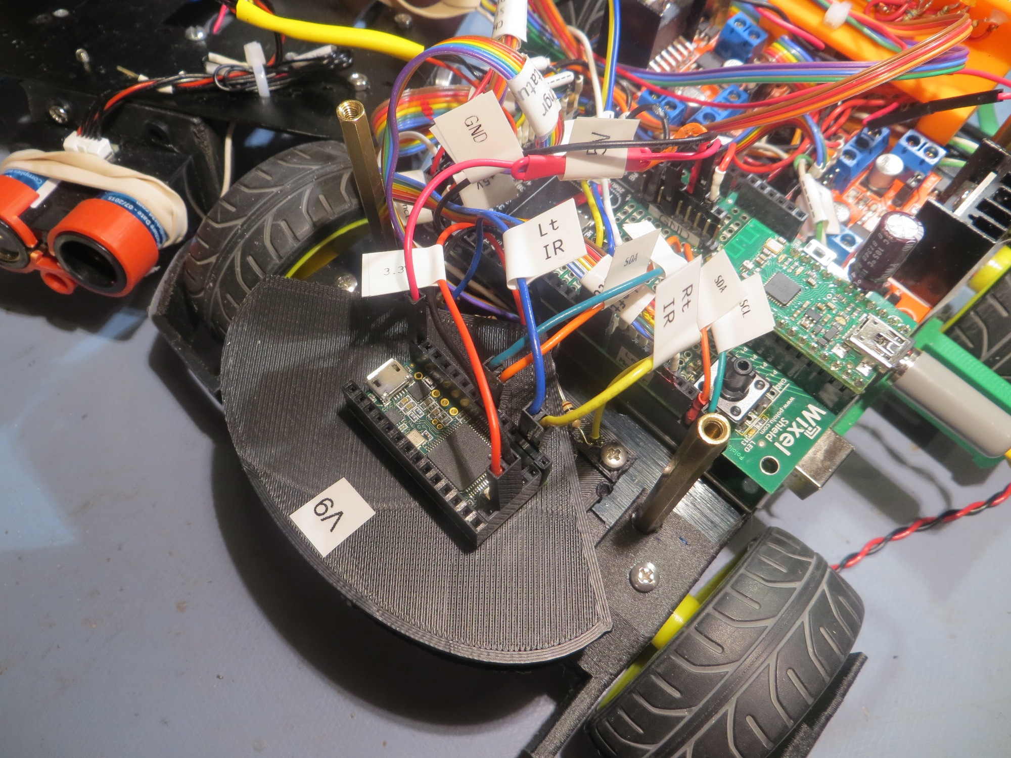
The Hardware:
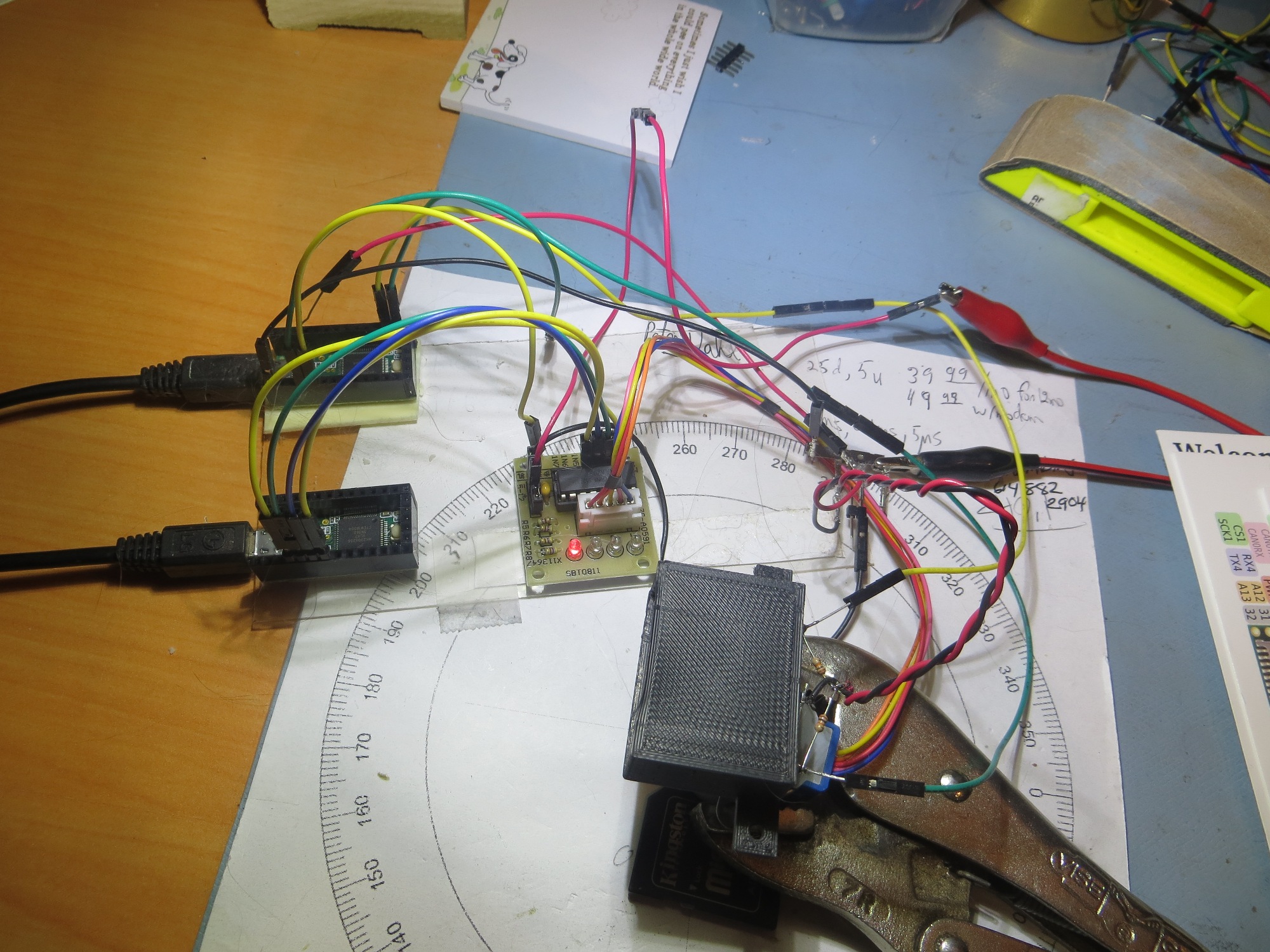
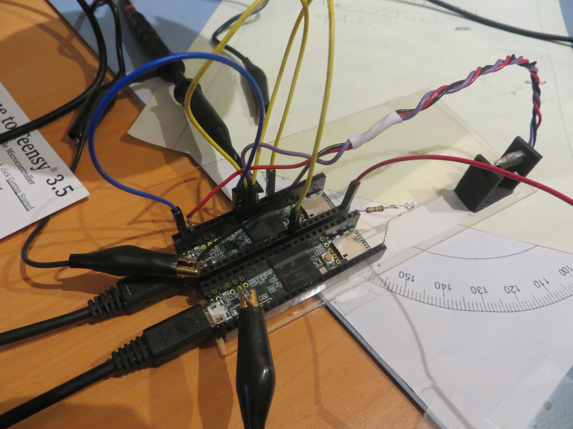
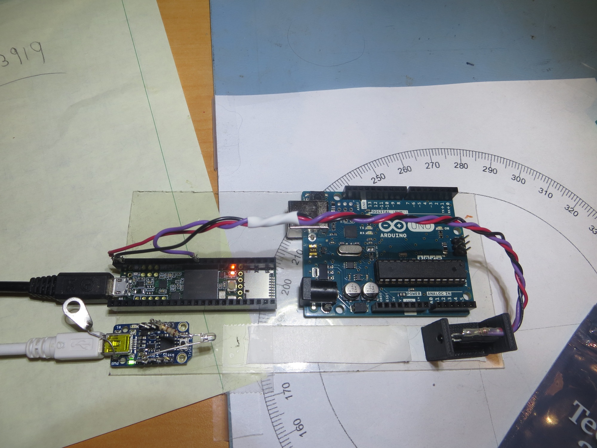
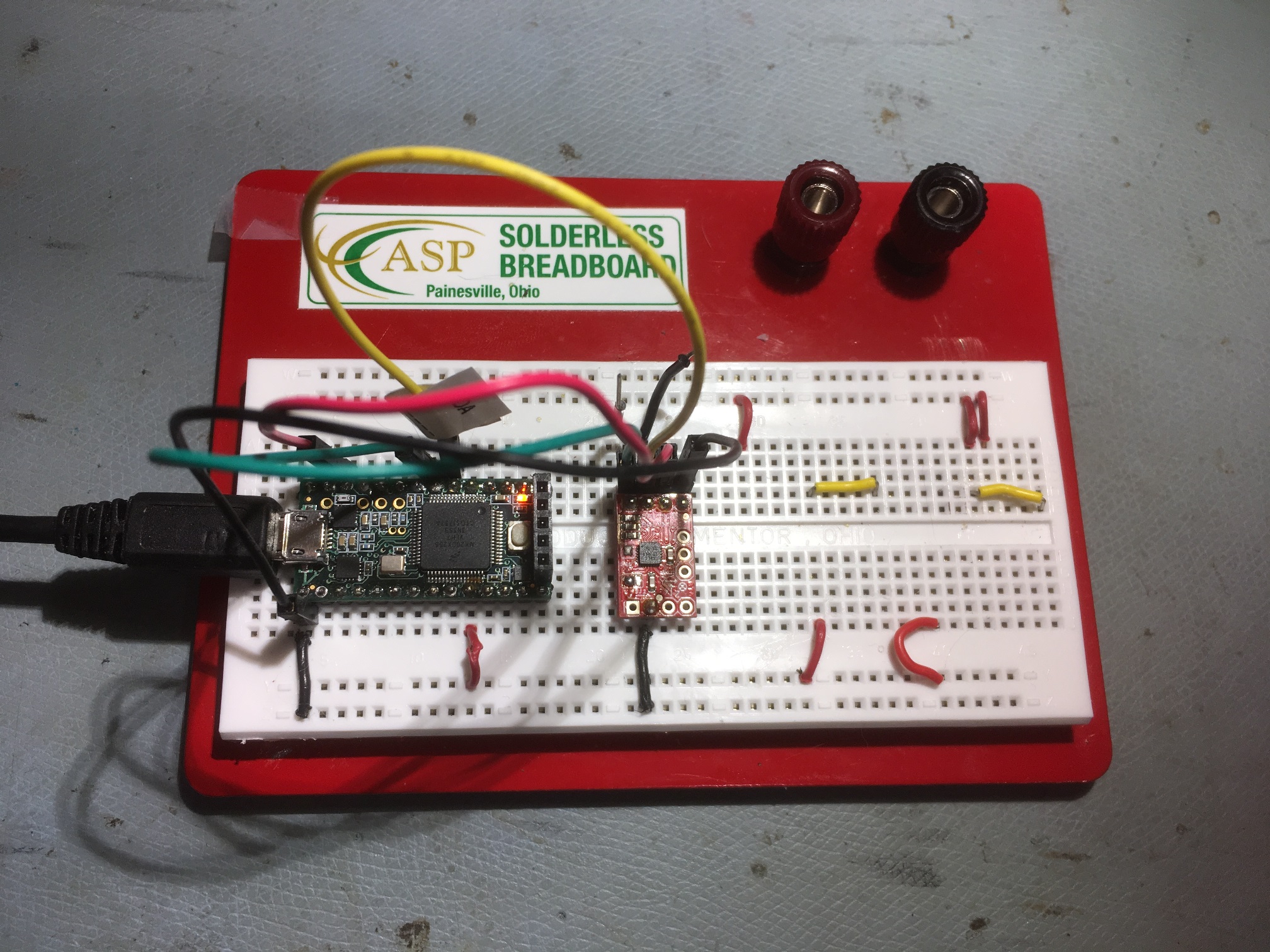
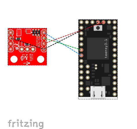
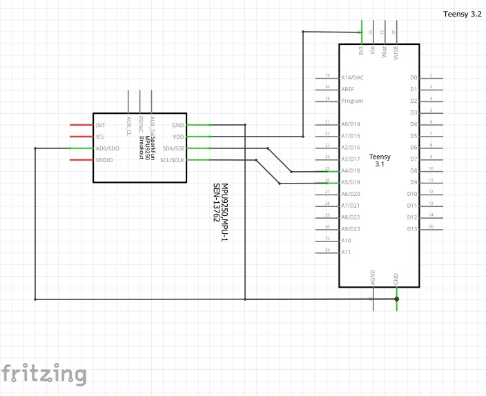
I used a Teensy 3.2 and a Sparkfun MPU 9250 IMU breakout board, both mounted on a small ASP solderless breadboard, as shown in the following photo, along with a Fritzing view of the layout
The Software:
I wrote a short program to display heading (yaw) values from the 9250, as shown below. The program uses Brian (nox771)’s wonderful i2c_t3 I2C library for the Teensy 3.x & LC controllers, and a modified version of ‘Class_MPU9250BasicAHRS_t3.h/cpp that incorporates an adaptation of Sebastian Madgwick’s “…efficient orientation filter” for 6D0F vs 9DOF. The modification removes the magnetometer information from the calculations, as I already know that the magnetic field in my environment is corrupted with house wiring and is unreliable.
|
1 2 3 4 5 6 7 8 9 10 11 12 13 14 15 16 17 18 19 20 21 22 23 24 25 26 27 28 29 30 31 32 33 34 35 36 37 38 39 40 41 42 43 44 45 46 47 48 49 50 51 52 53 54 55 56 57 58 59 |
/* Name: Teensy_MPU9250_Test.ino Created: 9/15/2019 11:46:10 AM Author: FRANKWIN10\Frank */ /* All this program does is display heading values from a Sparkfun MPU9250 breakout board at the default (0x68) I2C address. Note that it uses a slightly modified version of Class_MPU9250BasicAHRS_t3.h/cpp that incorporates an adaptation of Sebastian Madgwick's "...efficient orientation filter" for 6D0F vs 9DOF. The modification removes the magnetometer information from the calculations, as I already know that the magnetic field in my environment is corrupted with house wiring and is unreliable. */ #include "Class_MPU9250BasicAHRS_t3.h" //extracted all #defines from MPU9250BasicAHRS_t3.ino #include <i2c_t3.h> #include <elapsedMillis.h> elapsedMillis sinceLastPrint; Class_MPU9250BasicAHRS myIMU; int pulsePin = LED_BUILTIN;//04/10/18 added per-step pulse pin parameter bool bFirstTime = true; const long MSEC_PER_PRINT = 100; void setup() { Serial.begin(115200); delay(3000); //delay required to wait for Serial object creation //Wire.begin(); pinMode(LED_BUILTIN, OUTPUT); Wire.begin(I2C_MASTER, 0x00, I2C_PINS_18_19, I2C_PULLUP_EXT, 400000); //Wire.begin(I2C_MASTER, 0x00, I2C_PINS_18_19, I2C_PULLUP_INT, 400000); Wire.setDefaultTimeout(200000); // 200ms //IMU init & test Serial.println("Starting program..."); Serial.println("Initializing 9250 IMU..."); myIMU.init9250IMU(); Serial.println("Done..."); } void loop() { float hdg_deg = myIMU.GetIMUHeadingDeg(); if (bFirstTime) { bFirstTime = false; Serial.printf("Msec\tHdg\n"); } if (sinceLastPrint > MSEC_PER_PRINT) { Serial.printf("%lu\t%4.2f\n", millis(), hdg_deg); sinceLastPrint -= MSEC_PER_PRINT; } } |
The modified Madgwick routine is included below
|
1 2 3 4 5 6 7 8 9 10 11 12 13 14 15 16 17 18 19 20 21 22 23 24 25 26 27 28 29 30 31 32 33 34 35 36 37 38 39 40 41 42 43 44 45 46 47 48 49 50 51 52 53 54 55 56 57 58 59 60 61 62 63 64 65 66 67 68 69 70 71 72 73 74 75 76 77 78 79 80 81 82 83 84 85 86 87 88 89 90 91 92 93 94 95 96 97 98 99 100 101 102 103 104 105 106 107 108 109 110 111 112 113 114 115 116 117 118 119 120 121 122 123 124 125 126 127 128 129 130 131 132 133 134 135 136 137 138 139 140 141 142 143 144 145 146 147 148 149 150 151 152 153 154 155 156 157 158 159 160 161 162 163 164 165 166 167 168 169 170 171 172 173 174 175 176 177 178 179 180 181 182 183 184 185 186 187 188 189 190 191 192 193 194 195 196 197 198 199 200 201 202 203 204 205 206 207 208 209 210 211 212 213 214 215 216 217 218 219 220 221 222 223 224 225 226 227 228 229 230 231 232 233 234 235 236 237 238 239 240 241 242 243 244 245 246 247 248 249 250 251 252 253 254 255 256 257 258 259 260 261 262 263 264 265 266 267 268 269 270 271 272 273 274 275 276 |
// Implementation of Sebastian Madgwick's "...efficient orientation filter for... inertial/magnetic sensor arrays" // (see http://www.x-io.co.uk/category/open-source/ for examples and more details) // which fuses acceleration and rotation rate to produce a quaternion-based estimate of relative // device orientation -- which can be converted to yaw, pitch, and roll. Useful for stabilizing quadcopters, etc. // The performance of the orientation filter is at least as good as conventional Kalman-based filtering algorithms // but is much less computationally intensive---it can be performed on a 3.3 V Pro Mini operating at 8 MHz! void Class_MPU9250BasicAHRS::MadgwickQuaternionUpdate(float ax, float ay, float az, float gx, float gy, float gz) //void Class_MPU9250BasicAHRS::MadgwickQuaternionUpdate(float ax, float ay, float az, float gx, float gy, float gz, float q_array[4], float delta_t) { float q1 = q[0], q2 = q[1], q3 = q[2], q4 = q[3]; // short name local variable for readability //float q1 = q_array[0], q2 = q_array[1], q3 = q_array[2], q4 = q_array[3]; // short name local variable for readability float norm; // vector norm float f1, f2, f3; // objetive funcyion elements float J_11or24, J_12or23, J_13or22, J_14or21, J_32, J_33; // objective function Jacobian elements float qDot1, qDot2, qDot3, qDot4; float hatDot1, hatDot2, hatDot3, hatDot4; float gerrx, gerry, gerrz, gbiasx, gbiasy, gbiasz; // gyro bias error // Auxiliary variables to avoid repeated arithmetic float _halfq1 = 0.5f * q1; float _halfq2 = 0.5f * q2; float _halfq3 = 0.5f * q3; float _halfq4 = 0.5f * q4; float _2q1 = 2.0f * q1; float _2q2 = 2.0f * q2; float _2q3 = 2.0f * q3; float _2q4 = 2.0f * q4; //04/24/18 bugfix: these vars aren't used in 6DOF version //float _2q1q3 = 2.0f * q1 * q3; //float _2q3q4 = 2.0f * q3 * q4; // Normalise accelerometer measurement norm = sqrt(ax * ax + ay * ay + az * az); if (norm == 0.0f) return; // handle NaN norm = 1.0f / norm; ax *= norm; ay *= norm; az *= norm; // Compute the objective function and Jacobian f1 = _2q2 * q4 - _2q1 * q3 - ax; f2 = _2q1 * q2 + _2q3 * q4 - ay; f3 = 1.0f - _2q2 * q2 - _2q3 * q3 - az; J_11or24 = _2q3; J_12or23 = _2q4; J_13or22 = _2q1; J_14or21 = _2q2; J_32 = 2.0f * J_14or21; J_33 = 2.0f * J_11or24; // Compute the gradient (matrix multiplication) hatDot1 = J_14or21 * f2 - J_11or24 * f1; hatDot2 = J_12or23 * f1 + J_13or22 * f2 - J_32 * f3; hatDot3 = J_12or23 * f2 - J_33 * f3 - J_13or22 * f1; hatDot4 = J_14or21 * f1 + J_11or24 * f2; // Normalize the gradient norm = sqrt(hatDot1 * hatDot1 + hatDot2 * hatDot2 + hatDot3 * hatDot3 + hatDot4 * hatDot4); hatDot1 /= norm; hatDot2 /= norm; hatDot3 /= norm; hatDot4 /= norm; // Compute estimated gyroscope biases gerrx = _2q1 * hatDot2 - _2q2 * hatDot1 - _2q3 * hatDot4 + _2q4 * hatDot3; gerry = _2q1 * hatDot3 + _2q2 * hatDot4 - _2q3 * hatDot1 - _2q4 * hatDot2; gerrz = _2q1 * hatDot4 - _2q2 * hatDot3 + _2q3 * hatDot2 - _2q4 * hatDot1; // Compute and remove gyroscope biases //04/24/18 bugfix: gbias vars are unitialized here //gbiasx += gerrx * deltat_sec * zeta; //gbiasy += gerry * deltat_sec * zeta; //gbiasz += gerrz * deltat_sec * zeta; gbiasx = gerrx * deltat_sec * zeta; gbiasy = gerry * deltat_sec * zeta; gbiasz = gerrz * deltat_sec * zeta; gx -= gbiasx; gy -= gbiasy; gz -= gbiasz; // Compute the quaternion derivative qDot1 = -_halfq2 * gx - _halfq3 * gy - _halfq4 * gz; qDot2 = _halfq1 * gx + _halfq3 * gz - _halfq4 * gy; qDot3 = _halfq1 * gy - _halfq2 * gz + _halfq4 * gx; qDot4 = _halfq1 * gz + _halfq2 * gy - _halfq3 * gx; // Compute then integrate estimated quaternion derivative q1 += (qDot1 - (beta * hatDot1)) * deltat_sec; q2 += (qDot2 - (beta * hatDot2)) * deltat_sec; q3 += (qDot3 - (beta * hatDot3)) * deltat_sec; q4 += (qDot4 - (beta * hatDot4)) * deltat_sec; // Normalize the quaternion norm = sqrt(q1 * q1 + q2 * q2 + q3 * q3 + q4 * q4); // normalise quaternion norm = 1.0f / norm; q[0] = q1 * norm; q[1] = q2 * norm; q[2] = q3 * norm; q[3] = q4 * norm; } float Class_MPU9250BasicAHRS::GetIMUHeadingDeg() { // If intPin goes high, all data registers have new data //if (readByte(MPU9250_ADDRESS, INT_STATUS) & 0x01) { // On interrupt, check if data ready interrupt readAccelData(accelCount); // Read the x/y/z adc values getAres(); // Now we'll calculate the accleration value into actual g's ax = (float)accelCount[0] * aRes; // - accelBias[0]; // get actual g value, this depends on scale being set ay = (float)accelCount[1] * aRes; // - accelBias[1]; az = (float)accelCount[2] * aRes; // - accelBias[2]; readGyroData(gyroCount); // Read the x/y/z adc values getGres(); // Calculate the gyro value into actual degrees per second gx = (float)gyroCount[0] * gRes; // get actual gyro value, this depends on scale being set gy = (float)gyroCount[1] * gRes; gz = (float)gyroCount[2] * gRes; #ifndef NO_MAG readMagData(magCount); // Read the x/y/z adc values getMres(); magbias[0] = +470.; // User environmental x-axis correction in milliGauss, should be automatically calculated magbias[1] = +120.; // User environmental x-axis correction in milliGauss magbias[2] = +125.; // User environmental x-axis correction in milliGauss // Calculate the magnetometer values in milliGauss // Include factory calibration per data sheet and user environmental corrections mx = (float)magCount[0] * mRes*magCalibration[0] - magbias[0]; // get actual magnetometer value, this depends on scale being set my = (float)magCount[1] * mRes*magCalibration[1] - magbias[1]; mz = (float)magCount[2] * mRes*magCalibration[2] - magbias[2]; #endif // !NO_MAG } Now = micros(); deltat_sec = ((Now - lastUpdate) / 1000000.0f); // set integration time by time elapsed since last filter update lastUpdate = Now; sum += deltat_sec; // sum for averaging filter update rate sumCount++; // Sensors x (y)-axis of the accelerometer is aligned with the y (x)-axis of the magnetometer; // the magnetometer z-axis (+ down) is opposite to z-axis (+ up) of accelerometer and gyro! // We have to make some allowance for this orientationmismatch in feeding the output to the quaternion filter. // For the MPU-9250, we have chosen a magnetic rotation that keeps the sensor forward along the x-axis just like // in the LSM9DS0 sensor. This rotation can be modified to allow any convenient orientation convention. // This is ok by aircraft orientation standards! // Pass gyro rate as rad/s #ifndef NO_MAG MadgwickQuaternionUpdate(ax, ay, az, gx*PI / 180.0f, gy*PI / 180.0f, gz*PI / 180.0f, my, mx, mz); // MahonyQuaternionUpdate(ax, ay, az, gx*PI/180.0f, gy*PI/180.0f, gz*PI/180.0f, my, mx, mz); #else //Serial.printf("q = {%4.2f, %4.2f, %4.2f, %4.2f, deltat_ms = %2.4f\n", q[0], q[1], q[2], q[3], deltat_sec*1000); //experiment with multiple iterations on quat update //for (size_t i = 0; i < 10; i++) { MadgwickQuaternionUpdate(ax, ay, az, gx*PI / 180.0f, gy*PI / 180.0f, gz*PI / 180.0f); } //MadgwickQuaternionUpdate(ax, ay, az, gx*PI / 180.0f, gy*PI / 180.0f, gz*PI / 180.0f, q, deltat_sec); #endif // !NO_MAG if (!AHRS) { delt_t = millis() - count; if (delt_t > 500) { if (SerialDebug) { // Print acceleration values in milligs! Serial.print("X-acceleration: "); Serial.print(1000 * ax); Serial.print(" mg "); Serial.print("Y-acceleration: "); Serial.print(1000 * ay); Serial.print(" mg "); Serial.print("Z-acceleration: "); Serial.print(1000 * az); Serial.println(" mg "); // Print gyro values in degree/sec Serial.print("X-gyro rate: "); Serial.print(gx, 3); Serial.print(" degrees/sec "); Serial.print("Y-gyro rate: "); Serial.print(gy, 3); Serial.print(" degrees/sec "); Serial.print("Z-gyro rate: "); Serial.print(gz, 3); Serial.println(" degrees/sec"); #ifndef NO_MAG // Print mag values in degree/sec Serial.print("X-mag field: "); Serial.print(mx); Serial.print(" mG "); Serial.print("Y-mag field: "); Serial.print(my); Serial.print(" mG "); Serial.print("Z-mag field: "); Serial.print(mz); Serial.println(" mG"); tempCount = readTempData(); // Read the adc values temperature = ((float)tempCount) / 333.87 + 21.0; // Temperature in degrees Centigrade // Print temperature in degrees Centigrade Serial.print("Temperature is "); Serial.print(temperature, 1); Serial.println(" degrees C"); // Print T values to tenths of s degree C #endif // !NO_MAG } count = millis(); } } else { // Serial print and/or display at 0.5 s rate independent of data rates delt_t = millis() - count; //if (delt_t > 500) { // update LCD once per half-second independent of read rate if (SerialDebug) { Serial.print("ax = "); Serial.print((int)1000 * ax); Serial.print(" ay = "); Serial.print((int)1000 * ay); Serial.print(" az = "); Serial.print((int)1000 * az); Serial.println(" mg"); Serial.print("gx = "); Serial.print(gx, 2); Serial.print(" gy = "); Serial.print(gy, 2); Serial.print(" gz = "); Serial.print(gz, 2); Serial.println(" deg/s"); #ifndef NO_MAG Serial.print("mx = "); Serial.print((int)mx); Serial.print(" my = "); Serial.print((int)my); Serial.print(" mz = "); Serial.print((int)mz); Serial.println(" mG"); #endif // !NO_MAG Serial.print("q0 = "); Serial.print(q[0]); Serial.print(" qx = "); Serial.print(q[1]); Serial.print(" qy = "); Serial.print(q[2]); Serial.print(" qz = "); Serial.println(q[3]); } // Define output variables from updated quaternion---these are Tait-Bryan angles, commonly used in aircraft orientation. // In this coordinate system, the positive z-axis is down toward Earth. // Yaw is the angle between Sensor x-axis and Earth magnetic North (or true North if corrected for local declination, looking down on the sensor positive yaw is counterclockwise. // Pitch is angle between sensor x-axis and Earth ground plane, toward the Earth is positive, up toward the sky is negative. // Roll is angle between sensor y-axis and Earth ground plane, y-axis up is positive roll. // These arise from the definition of the homogeneous rotation matrix constructed from quaternions. // Tait-Bryan angles as well as Euler angles are non-commutative; that is, the get the correct orientation the rotations must be // applied in the correct order which for this configuration is yaw, pitch, and then roll. // For more see http://en.wikipedia.org/wiki/Conversion_between_quaternions_and_Euler_angles which has additional links. yaw = atan2(2.0f * (q[1] * q[2] + q[0] * q[3]), q[0] * q[0] + q[1] * q[1] - q[2] * q[2] - q[3] * q[3]); pitch = -asin(2.0f * (q[1] * q[3] - q[0] * q[2])); roll = atan2(2.0f * (q[0] * q[1] + q[2] * q[3]), q[0] * q[0] - q[1] * q[1] - q[2] * q[2] + q[3] * q[3]); pitch *= 180.0f / PI; yaw *= 180.0f / PI; //yaw -= 13.8; // Declination at Danville, California is 13 degrees 48 minutes and 47 seconds on 2014-04-04 roll *= 180.0f / PI; if (SerialDebug) { Serial.print("Yaw, Pitch, Roll: "); Serial.print(yaw, 2); Serial.print(", "); Serial.print(pitch, 2); Serial.print(", "); Serial.println(roll, 2); Serial.print("rate = "); Serial.print((float)sumCount / sum, 2); Serial.println(" Hz"); } //Serial.printf("%3.2f\t%3.2f\t%3.2f\n", yaw, pitch, roll); // With these settings the filter is updating at a ~145 Hz rate using the Madgwick scheme and // >200 Hz using the Mahony scheme even though the display refreshes at only 2 Hz. // The filter update rate is determined mostly by the mathematical steps in the respective algorithms, // the processor speed (8 MHz for the 3.3V Pro Mini), and the magnetometer ODR: // an ODR of 10 Hz for the magnetometer produce the above rates, maximum magnetometer ODR of 100 Hz produces // filter update rates of 36 - 145 and ~38 Hz for the Madgwick and Mahony schemes, respectively. // This is presumably because the magnetometer read takes longer than the gyro or accelerometer reads. // This filter update rate should be fast enough to maintain accurate platform orientation for // stabilization control of a fast-moving robot or quadcopter. Compare to the update rate of 200 Hz // produced by the on-board Digital Motion Processor of Invensense's MPU6050 6 DoF and MPU9150 9DoF sensors. // The 3.3 V 8 MHz Pro Mini is doing pretty well! digitalWrite(myLed, !digitalRead(myLed)); count = millis(); sumCount = 0; sum = 0; } } return yaw; } |
Note to self; after reviewing the extensive email thread with Kris Winer (tleracorp@gmail.com) I now believe I encapsulated all the required modifications to the AHRS code into a new class called “Class_MPU9250BasicAHRS_t3” with Class_MPU9250BasicAHRS_t3.h & .cpp files, and then referenced this new class in my MPU9250 work.
The results:
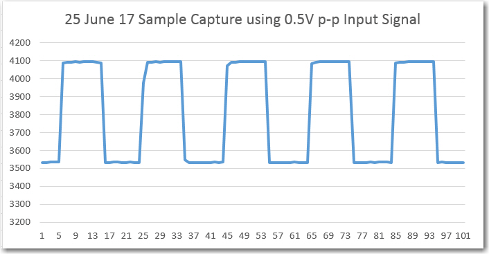
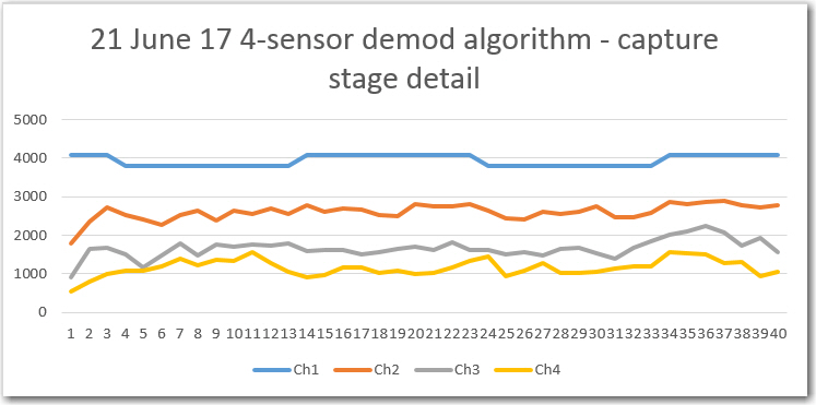
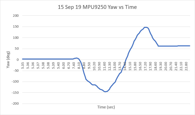
After getting everything working (and figuring out the history), I finally started getting reliable heading data from the MPU9250 as shown in the following Excel plot, where the breadboard was manually rotated back and forth.
Stay tuned,
Frank