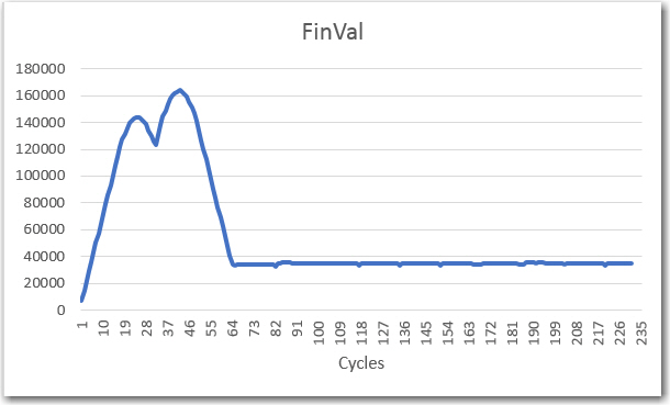
Yearly Archives: 2017

IR Modulation Processing Algorithm Development. Part XV

Posted 18 July 2017,

In my last post on this (somewhat long-winded) subject, I described the implementation of a Teensy-based sweep generator utility for use in testing the band-pass filter (BPF) application, and showed some results from the 52Hz version of the BPF.  As a result of this work, I believe I had validated both the test instrumentation and the 52Hz BPF implementation.

This post extends the previous work to the original goal for this project – the 520Hz BPF implementation.  When I did the original work on the 520Hz version, it was clear there was  something wrong, but not what.  For reference, here are some representative plots from this 24 June 2017 post.

Computed final values vs complete input data cycles for sensor channel 1

There has been a  lot of water over the dam between the 24 June post and now.

  • Replaced Trinket-based square-wave generator with Teensy 3.5 one for better frequency stability/accuracy
  • Replaced simple square-wave generator with frequency/amplitude sweep generator
  • Added ’round-trip’ measurement capability.  Sweep generator -> BPF -> sweep generator so BPF response can be directly correlated to sweep generator output.
  • Revised BPF code to eliminate all but one sensor channel
  • Replaced all in-line printouts with writes to internal arrays, with post-run printout option.
  • Added micro-second accuracy time stamps to demodulator internal data capture
  • Temporarily reduced filter center freq from 520Hz to 52Hz to eliminate any possibility of timing problems due to Teensy 3.5 internal interrupts.

As the plots from the previous post showed, the 52Hz BPF implementation works as intended.  So, it was time to try my hand (again!) with the 520Hz version.  First, I did an elapsed time study, to make sure no sample periods were being missed.  As the plot below shows, all the elapsed time values are reasonable, with only a few going to 101  Î¼Sec.  I speculate that the 101 values may be due to execution of extra-long internal Teensy ISRs.  The elapsed time plot conclusively demonstrates that  something I did during the above list of changes eliminated the occasional (1 out of 68 or 69 cycles) missed sample that caused the previous ‘crappy’ results for the 520Hz version of the filter. My personal favorite for the culprit is one or more of the print statements I had in the original code for debugging.

Sample times vs time.

The next set of plots shows the results of an amplitude sweep, with the amplitude set to a fixed 50% p-p value

‘raw’ Final Values vs time, with fixed frequency, 50% p-p

’round-trip’ Final Values vs time, fixed freq, 50% p-p

detail of ‘raw’ pot

The above plots weren’t quite what I expected; both the ‘raw’ and ’round-trip’ final values were lower than expected, and the ‘raw’ plot had a  lot more ripple than I wanted to see.  This all led me to believe that the test frequency was not centered in the BPF passband.  I had not actually double-checked this, so I went back a few steps and made sure the fixed amplitude sweep frequency was indeed synched with the demodulator sampling frequency.  After that, the plots got a lot cleaner, as shown below.

‘raw’ final values vs time after synching Tx & Rx frequencies


In the above plot, the ‘raw’ final value is pretty steady around the value 1,320,000, which agrees well with a 50% p-p Tx level.

Next, I ran frequency sweeps, as shown in the following plots

‘raw’ Final Values vs frequency, with amplitude @ 50% p-p

’round-trip’ Final Values vs frequency, with amplitude @ 50% p-p

For reference, the same two plots for the 52Hz implementation are shown below

Captured ‘raw’ final value from IR demodulator. Frequency values added later

Frequency sweep results from sweep generator printout (D/A from IR demod, then A/D in sweep gen)

Next, I ran an amplitude sweep from 0% to 100% p-p input, as shown in the following plots

‘raw’ Final Values vs amplitude, with frequency @ 520.8Hz

’round-trip’ Final Values vs amplitude, with frequency @ 520.8Hz

So, it appears to me that the 520Hz BPF is working just as well as the 52Hz one, and it’s time to move on to multi-sensor operation.

I have placed the code for the now working 52/520Hz single-channel N-path BPF on GitHub at  https://github.com/paynterf/SqWaveIQDemodV2.git.  There are three branches available on GitHub, as follows:

  1. Master – this is the original ‘root’ for the IQ Demodulator (BPF) project
  2. SingleChannel – this is the final code for the single channel version, working at 52 & 520Hz
  3. TwoChannel – this is my new branch to host the in-progress dual-channel BPF.

Stay tuned!

Frank


IR Modulation Processing Algorithm Development. Part XIV

Posted 07 July 2017

In my last post on this subject, I described a working 52Hz implementation of John Jenkins’ ‘degenerate N-Path Band-pass filter (BPF).  This filter is intended to allow Wall-E2 (my wall-following robot) to discriminate between the IR homing beam from a charging station and other ambient IR interferers.  This post describes the implementation of a basic swept-frequency square-wave function generator for use in testing BPF performance.

Now that I have a working (I think) version of the BPF algorithm, I want to implement and test a frequency and amplitude sweeping module so I can use it to test not only the working 52Hz BPF implementation, but the (so far not working) 520Hz implementation when we finally get the bugs worked out of it.   My idea is that doing this now will have two (maybe three) significant benefits

  • Allows me to fully characterize the existing 52Hz BPF implementation
  • Gives me baseline performance characteristics for comparison against 520Hz results
  • (freebie) – More fun with Teensy!

I’m already using a second Teensy 3.5 as the 52Hz square wave transmitter in my test setup, so all I need to do is to modify the existing program to sweep the desired frequencies and amplitudes.  I think I’ll do this as a command-line parameter-entry program, with user-entry parameters for  start, stop, and step frequencies (Hz) and fixed amplitude (% full-scale) for the frequency sweep module, and  start, stop, and step amplitudes (% full-scale) and a set center freq for the amplitude sweep module.

12-15 July 2017 Update:

Well, I finally got the sweep generator going, at least the frequency sweep part, and managed to get some good data out of the 52Hz square wave demodulator.  What I was striving for was something akin to the normal hardware setup where a frequency-sensitive ‘device under test’ (DUT) is driven from a frequency sweep generator, and a data logger of some sort records the result, something like the following block diagram.  Back in the day, the ‘datalogger’ was quite often an engineer recording results on a piece of graph paper – how quaint!  😉

Typical swept frequency test setup

In this project, the DUT is the Teensy 3.5 hosting the IR demodulator code, and the frequency sweep generator is another Teensy 3.5 hosting the code to generate a swept-frequency square wave signal.

But, what to do about the datalogger?  I could record data from inside the demodulator program, but we’re talking a  lot of data; even at 52Hz that’s 52 4-byte values per second, and a sweep test might take as long as 3 minutes –> 36000 bytes.  Fortunately, the Teensy 3.x sports 192KB of RAM, so a 36KB chunk barely scratches the paint – yay!!  Another problem with logging internal to the demod module is how to correlate the captured data with the driving frequency; they are obviously correlated, but it’s not a slam-dunk to unequivocally assign particular frequencies to a particular stored data value.

So, I decided on a two-pronged approach; I will indeed save the data internally to RAM for later printout, but will also output an appropriately scaled version of the ‘final value’ calculation to one of the two DAC ports available on the Teensy 3.5 SBC.  I plan to run this signal back to the sweep generator module so I can correlate ‘final value’ values with test frequencies, as shown in the following amended block diagram.

Modified sweep test block diagram

This setup works, and now I can get frequency-correlated ‘final value’ data  from the sweep generator A/D.  However, since the demodulator module ‘free-runs’ with respect to the sweep generator, the final value storage array can fill up before the frequency sweep finishes (or even before it starts!), so something is needed to synch the two modules.  As the following block diagram shows, this is accomplished by providing a digital trigger from the sweep generator to start the demodulator.  Also added in this final setup is the ability to set the square wave amplitude, for later amplitude sweep tests (set to 50% amplitude for the swept-frequency tests)

Final sweep setup. Note DAC block for square wave amplitude adjustment and trigger signal for synchronization

With the above setup I ran a number of frequency sweeps, as shown in the plots below.  I started out with a sweep from 48 to 56Hz (+/- 4Hz from center freq), but quickly narrowed it down to +/- 2Hz.  As my friend and mentor John Jenkins pointed out in his gentle, diplomatic way (something like “What  were you  thinking!“), the BPF bandwith is less than 1Hz, so a +/- 4Hz sweep range will just record a lot of nothing – oops!

Frequency sweep results from sweep generator printout (D/A from IR demod, then A/D in sweep gen)

Captured ‘raw’ final value from IR demodulator. Frequency values added later

Even though the above sweeps were way too wide, it is clear that the demodulator algorithm is working (at least in the 52Hz implementation).

Frequency sweep results from sweep generator printout (D/A from IR demod, then A/D in sweep gen)

Captured ‘raw’ final value from IR demodulator. Frequency values added later

In the above plots, the sweep was reduced to +/- 2Hz, and the number of steps increased to 80.  The result is a much more detailed look at the BPF response.  As expected the general shape of the ’round-trip’ (individual ‘final value’ numbers sent from the demodulator to the sweep generator via the DAC-A/D channel and then printed) plot and the ‘raw final value’ plot match, but I didn’t expect either the flat-top region at the center of both plots or the fine ripple shown in the ‘raw’ plot.  I made a number of additional sweeps with up to 160 steps at 2 sec/step, but neither the flat-top region nor the fine ripple features changed – they are apparently real features of the BPF response.

I think I finally figured out that the flat-top region was due to the fact that there is a narrow range of frequencies for which the filter response is maximum and identical.  In this very narrow region, the digital sample points are ‘perfectly’ aligned with the incoming square wave, so that the final value is the maximum possible value for the input p-p amplitude.

As for the fine ripple features, I think these are due to the beat frequency between the incoming signal and the sample period.  If this is the case, I would expect the ripple features to be more closely spaced far away from the center frequency, and less closely spaced toward the center. This certainly seems to be the case in the above plot, but even more evident in the detail plots below, (points extracted from the main plot above)

far and near center BPF response detail

Next, I performed an amplitude sweep from 100% to 0% p-p amplitude, with the center frequency set to 51.87Hz (this value was empirically determined earlier), with the following results

‘Raw’ final values from amplitude sweep.

final values captured by sweep generator

As the above plots show, the filter response is very linear with respect to p-p amplitude variations.  The maximum value shown in the ‘raw’ plot above is a little above 2.5 x 10⁶. The actual maximum value from the data is 2,606,752, which matches well with the theoretical maximum value of 4096*10*64 = 2,621,440.

Lastly, I performed another frequency sweep, but this time with a running-sum length of 32 cycles vs 64, to see how much the band-pass width was affected by halving the number of cycles in the running-sum circular buffer.  Comparing the 32-cycle and 64-cycle plots as shown below, the ‘flat-top bandwidth is considerably wider than the original 64-cycle sweep results  – about 1.8Hz edge-to-edge for 32 and about 0.4 for the original 64 version.  Maybe as much as 4x bandwidth increase.

Frequency sweep results from sweep generator printout (D/A from IR demod, then A/D in sweep gen)

Frequency sweep results from sweep generator printout (D/A from IR demod, then A/D in sweep gen)

Captured ‘raw’ final value from IR demodulator.

Summary and Conclusions:

This post described my efforts to characterize the frequency and amplitude responses for the 52Hz implementation of the ‘degenerate N-path band-pass filter’ described to me by friend and mentor John Jenkins some time ago.

The original plan was to use this filter technique at 520Hz to enable my Wall-E2 wall-following robot to home to a charging station using a square-wave modulated IR signal to suppress ambient IR interference.  Unfortunately, I could not get the 520Hz implementation to work properly, probably due to some unknown timing issues associated with the Teensy 3.x architecture.  So, I decided to run the filter at 1/10th speed (52Hz) instead, thereby eliminating any timing issues, and allowing me to establish a baseline for subsequent higher-speed testing.

As the data above shows, the effort to implement the N-path BPF at 52Hz was completely successful.  Both the frequency and amplitude responses were characterized.  In addition:

  • I gained a  lot more experience with the Teensy 3.x line of SBCs.  They are less than half the size of an Arduino Uno, have over 10x more RAM, 50x faster, come with on-board SD (3.5 & 3.6) cost about the same, and have about the same power requirements – such a deal!
  • Implemented a Teensy 3.5  frequency/amplitude sweep square wave generator, and verified proper operation by using it to characterize the 52Hz BPF implementation.
  • Implemented a Teensy 3.5  fixed-frequency square wave generator,  and verified proper operation by using it to find the correct transmit frequency for the 52Hz BPF implementation
  • Validated the efficacy of my little two-Teensy test bed.

The above tools can now be used with high confidence to investigate (and hopefully eliminate) the problems with running the BPF at 520Hz.

Stay tuned!

Frank


IR Modulation Processing Algorithm Development. Part XIII

Posted 03 July 2017

With this post, I’m nearing a new Personal Record for a subject series (the ‘Charging Station Design’ series went to 14), with no end in sight.  The last missive from my friend and mentor John Jenkins (I’m reconsidering the ‘friend’ part, as ASFAICT, he intends to drive me into an early grave over this project!) was ‘Still not there – the ‘Final Value’ output from the filter is still  wrong! :-(.

Be that as it may, it is my lot, challenge, ‘opportunity to excel’ or whatever, to continue working on this thing until I kill it – or it kills me (indeterminate as to which at the moment) 😉

So, after eliminating most/all of the print statements, John is still convinced that the Teensy is missing samples on a regular basis, and this is screwing up the rest of the algorithm.  I’m just as convinced that the Teensy is  way too fast to miss any samples, and that any problems must be later in the algorithm.

However, there may be a way to settle which is which, without the use of magic or a crystal ball.  The Teensy 3.5/3.6 SBC’s come with a built-in micro-SD card capability, which I think can be used to log  the output of each stage in a way that doesn’t (I hope) impact sample timing.

The first step in my new master plan is to make sure I can actually write to and read from an SD card on my demod Teensy (actually my first step was to go by MicroCenter and  get a micro-SD card, as all mine seem to have disappeared!).  I found and loaded    Paul Stoffregen’s nice little SD test sketch from his GitHub site, and ran it on my Teensy 3.5.  After changing the ‘chipSelect’ constant from the default 4 to ‘BUILTIN_SDCARD’, it ran successfully, and I was even able to open the ‘Test.txt’ on my PC – Yay!

The next step is to modify my IR demod program to send logging data to the SD card instead of the serial port, and to monitor my timing pulse output to make sure the SD card writes don’t interfere (can’t imagine they would, but I have a very limited imagination!).

After timing a loop that wrote 1000 short lines to the SD card, I reluctantly came to the conclusion that the stock SD card library may not be fast enough to ensure that logging output isn’t affecting the results of the algorithm.  There is a faster library (SdFat), and some other speedup techniques, but rather than going down yet another rabbit-hole, I decided it was time to try a different idea.

The original plan for the IR demod idea was to use a ~520Hz square-wave modulation frequency.  This is high enough to be well away from 60Hz line freq, and not aligned with higher line harmonics, but it may be just high enough to be causing the problems we are seeing.  Since the algorithm actually doesn’t care what the frequency is, I decided that I can put the timing issue to bed by simply reducing the modulation frequency by a factor of 10, to something like 52Hz.  Sample spacing at this frequency (assuming 20 samples/cycle) is 1000μS, which should provide more than enough room for computations (and hopefully some printouts).

To start this process, I modified both the transmit and receive Teensy 3.5 programs for the new, lower freq, and then tweaked the transmit frequency to synch with the receiver timing.  As the following short video shows, a transmit frequency of 51.87Hz and a receive frequency of 51.815Hz synched up fairly well.


The demodulator timing pulse train (the rising edge is at the start of the sampling/computation block,and the trailing edge is at the end) is shown in the following scope photos.

Bottom trace is sampler pulse train, top trace is square wave at ~52Hz. Time scale is 1ms/cm

Photo showing just one sampling period. Time scale is 0.1ms/cm

Expanded view of one sampling/computation period. Time scale is 5 microsec/cm

From the above photos, it is clear that the entire sampling/computation block takes less than 10μS, leaving about 990μS free before the next sample occurs.

Yesterday, ‘talking’ about this problem (‘talking’ with John can be a rather terrifying experience – sort of like ‘talking’ with Zeus – you wonder when the thunderbolt will arrive and whether or not he’s going to miss) with John, I opined that if his theory of missing samples is correct, a list of accurate sample timestamps should show some gaps; a linearly increasing timestamp value would refute the claim, and a plot with vertical jumps would validate it.

Then last night, as I was drifting off to sleep, I realized I didn’t have to actually  create the necessary timestamps, as I already had them in the code.  The elapsedMicros variable type such as ‘sinceLastSample’ gets incremented by the system each time through loop(), and only gets modified from inside the sampling/computation loop.  If  all  samples are taken on time, this variable should be a constant when measured inside the sample/computation block just before it gets reset.  The relevant code snippet is shown below

At the point shown by “/*RECORD sinceLastSample HERE!*/” in the above snippet, the ‘sinceLastSample’ variable should be  USEC_PER_SAMPLE +/- 1μS.  A dropped sample event should cause the value of this variable to change to N*USEC_PER_SAMPLE, where N is the number of consecutive dropped samples.

So, all I have to do is write the ‘sinceLastSample’ value to an array for a few seconds, and then write it back out again after stopping the program.  An Excel plot of the values should tell the tale, one way or the other

05 July 2017

Here are some preliminary results from the 52Hz implementation

A 2560-point (128 cycles) array containing ‘sinceLastSample’ values.

129-point array containing ‘Final Value’ values

Note that the ‘sinceLastSample’ value varies -0/+3  Î¼S from ideal (the actual value is something like  964.32  Î¼S), and there are clearly no dropped samples.

The ‘Final Value’ curve looks rather linear up to something like 680,000, which I suspect John is going to confirm is the correct value for a 0.8V p-p squarewave input at the center freq of the filter passband.

So, assuming John does indeed confirm the final value numbers are correct, pretty much validates the algorithm (unchanged from the 520Hz version), and lends credence to his idea that samples are getting dropped in the higher frequency implementation.

More to come,

Frank


IR Modulation Processing Algorithm Development. Part XII

Posted 01 July 2017

I went down a bit of a rabbit-hole between my last post on this subject and today.  I was attempting to run down the problems with my IR demodulation code when I discovered that the basic rate at which the demodulator captured samples was off by a factor of 5 or so – yikes!!  Instead of 20 samples per cycle, I was seeing more like 100, as shown below.

Raw data capture using ‘sinceLastOutput = 0’ in the first demodulation step

Raw data capture using ‘sinceLastOutput -= USEC_PER_SAMPLE’ in the first demodulation step

As you might expect, this development threw me for a bit of a loop – as the change from ‘sinceLastOutput = 0’ to ‘sinceLastOutput -= USEC_PER_SAMPLE’ was instrumental (or at least so I thought) to getting the transmit and receive frequencies matched more accurately.  So, now I had to go chase down yet another tangential problem – what I refer to as ‘going down a rabbit hole’. The only saving grace in all this is that, as a twice-retired engineer, I have no deadlines! 😉

To resolve this problem, I wound up creating an entirely new test program to isolate the issue, with just the following lines in the loop() function:

With the ‘sinceLastOutput -= USEC_PER_SAMPLE’ line active, I got about 100 samples/cycle. With this line commented out and the ‘sinceLastOutput = 0’ line active, I got the normal 20 samples/cycle, with nothing else being changed.

Once I was sure the test program was consistently producing the anomalous results I had noticed in the complete program, I posted this issue to the PJRC Forum, so I could get some help from the experts.  I knew it was something I was doing wrong – I just didn’t know  what!

Within a few hours I had received several responses, and the one that hit the bullseye was the one correctly identifying a subtlety with the the ‘-=’ elapsedMicros() usage format.  When this format is used, the accompanying ‘elapsedMicros’ variable must be initialized in the setup() code; otherwise it will be some arbitrary (and possibly quite large) value when the loop() function is first entered. This will cause the ‘if’ statement to trigger repeatedly until the ‘-=’ line eventually reduces the variable to a value below USEC_PER_SAMPLE, at which point it will start behaving as expected.  This odd behavior never happens with the ‘=0’ usage, as the variable is initialized on the first pass through the ‘if’ statement.  Sure enough, when I added a line at the bottom of my setup() function to set the ‘sinceLastOutput’ variable to zero, my little test program immediately stopped mis-behaving.

Well, this little side-journey only cost me a couple of days, and a few more white hairs (oh, wait –  my hair is already completely white – no problem!)  Back to my regularly scheduled program…

Frequency Matching:

My friend and mentor John Jenkins, who has been looking over my shoulder (and occasionally whacking me on the head) during this project, was unsure that my frequency matching setup was actually 100% complete, as the video I took the last time didn’t run long enough to convince him (and there were some un-explained triggering glitches as well).  So, I thought I would re-do this part to make him happy.  To do this I modified my little test program from the above ‘rabbit-hole’ elapsedMicros issue to output a square wave from the demodulator board that could be compared to the transmitter square wave.

As shown in the above video, the transmit and demodulator frequencies are quite well matched, showing essentially zero relative drift even over the 30-40 second time of the video.  Mission accomplished! ;-).

Sample Acquisition Step:

I modified my demodulator program to properly initialize the ‘elapsedMicros’ variable being used for sample timing, and verified proper operation by commenting out everything but the sample acquisition step.  I captured several hundred samples, and plotted the first hundred in Excel as follows:

100 samples using proper ‘elapsedMicros’ variable initialization

Sample Sum Step:

Next, each group of five samples (1/4 cycle) is summed, and the ‘In-phase’ and ‘Quadrature’ components are generated using the appropriate sign sequences.  As shown in the following, this appears to be happening correctly:

Cycle Sum Accumulation:

As each sample group is summed and the I/Q components generated, accumulate the 1/4-cycle I/Q sums into a ‘Cycle Sum’.  As the following printout shows, this step also is being performed properly


Running Sum Accumulation:

The last step in the algorithm is to compute the N-cycle running sum of all the cycle sums.  This is done by subtracting the oldest value from the circular buffer from the current running sum, adding the current cycle sum to the running sum, and then replacing the oldest cycle sum value in the circular buffer by the current cycle sum.

  1. RunningSum = RunningSum + CurrentCycleSum – OldestCycleSum
  2. OldestCycleSum = CurrentCycleSum
  3. Circular buffer index incremented by 1 (MOD N)

This one took a while to instrument properly. I first tried just adding some more columns on to the current display setup, but that became too cumbersome, too fast.  Verifying the running sum calculation requires looking at not only the current running sum, but also its value from N cycles (or N*5*4 samples) previously.  So, I modified the code to only print one line per cycle, and this was much easier to manage.  Here’s a partial printout showing a little over 200 cycles, representing about 400mSec (200 cycles * 2mSec/cycle).


To analyze these results, I dropped them into Excel, and used it’s ‘Freeze Panes’ feature to juxtapose the results from cycles 0 through 4 with cycles 65, 66, and 67.  This allowed me to verify that the running sum expression was being calculated correctly and the circular buffer was being loaded and referenced correctly.  When I finished verifying these results, I plotted the final value column, as shown below:


New ‘Final Value’ results

As an experiment, I also momentarily blocked the IR path with my finger, and plotted the results, as shown below:

Filter response with finger blocking IR path for a few seconds, then removed

And again, just waving my finger into and out of the IR path several times over several seconds

Filter response with finger moved in and out of IR path several times over 3-5 seconds

John’s comment on all this was “still not right”, as explained below:


“Think I misinterpreted earlier plot  as the one below makes it clearer what is happening.   The flat segments are when sample timing is proper.   So 3 good sets of cycles samplesin a row is max before there is a relative phase slip of ~1/10 of 180degs of Tx signal or ~96us = (time_for_180deg = (1/520)/2) / 10.
The slips are thus equal to  10 raw samples which are lost every ~35 Tx cycles = (51-16) for CSumQ  and ~34 Tx cycles (68-34) for CSumI.   So 20 raw samples (1 full Tx cycle)  are lost every  ~69 Tx cycles and this results in 64-cycle running I and Q sums being  only 5/64  of 64 times the actual  signal magnitude because all but  5 of the 64 values in running sums are canceled out by other values in the I and Q running sums.   Applying this to the running sum of abs(I)+abs(Q) gives ~35.8K which is close to what  you are seeing — that is:    ~35,823 = (5/64)*(64*7164.667)
Seems almost certain  that the calcs are correct and the problem is that the Teensy can’t keep up with the needed sample rate (probably due  coding approach or interrupts but less likely “magic timing code” Tx and Rx were very stable on scope).   Back to thinking ADC –> DMA may be the cure”

My take on the above was that it is the print statements that are the cause of the problem, not anything to do with Teensy ADC speed.  To test this theory, I removed all but the ‘Final Value’ print statement, and put that one statement in a block that executed only once per 64 cycles.  With this change, I could see that the print output was keeping up with real time and not lagging as before. Below shows a plot with several IR beam block/unblock cycles, and it appears that the ‘Final Value’ output is much more responsive to the block/unblock events.  Interestingly, it appears there is some sort of Gibbs phenomenon associated with the ‘fast’ cycles when the system switches between one equilibrium level and another.

The next step is to remove the print statements entirely and route the ‘Final Value’ output to one of the two DAC lines on the Teensy 3.5.  To test this idea, I adapted the HobbyTronics sine wave generator code to my project (pin A21 on the Teensy 3.5 vs A14 on the Teensy 3.2), and got the following display on my ‘scope:

Output from Teensy 3.5 DAC0 (A21) pin

So, now I know that the DAC output works – now I just need to scale the ‘Final Value’ numbers correctly and connect them to the DAC output.  Then I can watch the filter action in real time without worrying about the impact of print statements.

With an input square wave amplitude of about 0.35V p-p, or about 0.35/3.3 = 0.106 FS, the output is about 29,000.  Therefore the peak output from the FV stage should be about 29,000/0.106 ~ 273,584.  so an input of 0.35/3.3 = 0.106 should produce an output of (29,000/273584) *3.3 = 0.106*3.3 = 0.35

So, I modified my Sinewave test code to output the Final Value number, scaled by 273,584, and got the following display.  In this test, the input amplitude is about 0.35V p-p, and the output is about 0.35VDC


Stay tuned,

Frank


IR Modulation Processing Algorithm Development. Part XI

Posted 26 June 2017

In my last post on this subject, I had just decided to replace the Trinket transmit module with a second Teensy 3.5 to see if this would produce a more stable transmit waveform.  Indeed, it did seem to be more stable, as shown by the plots at the bottom of yesterday’s post.

Today I decided to see if I could further improve the situation by getting a closer match between the transmit and receive  frequencies.  To do this I modified the demodulator program to output a square wave at what it thinks is the right frequency, and compare it to the waveform being used to drive the IR LED.  If I can get these to match exactly, then there will still be a phase offset, but it will be a (mostly) constant factor.

The starting point for this effort is shown in the following short video, taken several eons (OK only 10 days) ago  on June 16.


With this as the starting point, I started first by tweaking the transmit frequency.  For this test, I triggered the scope on the receiver square wave signal, and tried to stop the drift of the transmit waveform.  After a while I got pretty close, but couldn’t get it stopped.  This was more than a little bit frustrating, as I thought the Teensy much higher clock speed should provide commensurately better resolution using the Teensy 3.x-specific ‘elapsedMicros’ type.

So, back to the inet for some more research.  After an hour or so I found this post, and buried in the middle of it was a reply by  PaulStoffregen    (creator of the Teensy line) that noted that

The proper way to get repeating on a 1000 us interval is this:

Code:

If you set “sinceLastRead” to zero, you could “lose” any increment it makes between the time your “if” condition runs and the time it’s written. An interrupt might occur, for example. By subtracting 1000, and increment it’s made will be preserved. Software latency can still cause jitter, but overall you’ll get the correct rate, even if interrupts delay the write to sinceLastRead.

I had been setting my elapsedMicros variable to zero, so I decided to try using Paul’s technique to see if the timing accuracy improved at all.  When I did, suddenly I was able to get the transmit and receive frequencies to match  very closely, as shown in the following short video clip


After seeing this miracle of timing, I decided to run another set of ‘final value’ plots in Excel, with the following results

These plots  seem a lot more consistent than before, and a lot less ‘spiky’, so maybe I’m making some progress.  However, friend and mentor John Jenkins’ comment was “still something wrong – magnitude is off” – rats! ;-).

Stay tuned,

Frank


IR Modulation Processing Algorithm Development. Part X

Posted 24 June 2017

Well, I may have spoken too soon about the perfection of my implementation of John’s ‘N-path’ band-pass filter (BPF) intended to make Wall-E2 impervious to IR interference.  After my last post on this subject, I re-ran some of the ‘Final Value’ plots for different received IR modulation amplitudes and the results were, to put it bluntly, crap 🙁 . Shown below is my original plot from yesterday, followed by the same plot for different input amplitudes

Computed final values vs complete input data cycles for sensor channel 1 (This is the original from yesterday)


So, clearly something is ‘fishy in Denmark’ here, when the ‘no-signal’ case with only high-frequency noise causes the output to increase without limit, and the ‘input grounded’ case is decidedly non-zero (although the values are  much lower than in the ‘signal present’ cases).

Time to go back through the entire algorithm (again!) looking for the problem(s).  

25 June 2017

My original implementation of the algorithm was set up to handle four sensor input channels, so each step of the process required an iteration step to go through all four, something like the code snippet below:

In order to simplify the debug problem, I decided to eliminate all these iteration steps and just focus on one channel.  To do this I ‘branched’ my project into a ‘SingleChannel’ branch using GIT and TortoiseGit’s wonderful GIT user interface (thanks TortoiseGit!).  This allows me to muck about in a new sandbox without completely erasing my previous work – yay!

Anyway, I eliminated all the 4-sensor iteration steps, and went back through each step to make sure each was operating properly.  When I was ‘finished’ (I never really finish with any program – I just tolerate whatever level of bugs or imperfections it has for some time).  After this, I ran some tests for proper operation using just one channel.  For these tests, the Teensy ADC channel being used was a) grounded, b) connected to 3.3VDC, c) unterminated.  For each condition I captured the ‘Final Value’ output from the algorithm and plotted it in Excel, as shown below.

Single channel testing with grounded, unterminated, and +3.3VDC input

As can be seen from the above plot, things seem to be working now, at least for a single channel.  The ‘grounded’ and ‘3.3VDC’ cases are very nearly zero for all time, as expected, and the ‘unterminated’ case is also very low.

Next, I added a 0.5V p-p signal at ~520Hz to the sensor input, and re-ran the program.  After capturing the ‘Final Value’ data as before, I added it to the above plot, as shown below

Final Value vs Cycles for 0.5V p-p input

As can be seen in the above plot, the ‘Final Value looks  much more reasonable than before. When plotted on the same scale as the ‘grounded’, ‘unterminated’, and ‘+3.3VDC’ conditions, it is clear that the 0.5V p-p case is a real signal.

Then I ran a much longer term (11,820 cycles, or about 22-23 sec) test with 0.5V p-p input, with the following results.

As can be seen from the above plot, the final value is a lot more ‘spiky’ than I expected.  The average value appears to be around 30,000, but the peaks are more like 60,000, an approximately 3:1 ratio.  With this sort of variation, I doubt that a simple thresholding operation for initial IR beam detection would have much chance of success.  Hopefully, these ‘spikes’ are an artifact of one or more remaining bugs in the algorithm, and they will go away once I find & fix them 😉

Update:  Noticed that there was a lot of time jitter on the received IR waveform – wonder if that is the cause of the spikes?

sensor waveform jitter. Note that this display is separately (Vert Mode) triggered.

Following up on this thread, I also looked at the IR LED (transmit) and photodetector (receive) waveforms together, and noted that there is quite a bit of time jitter on the Tx waveform as well, and this is received faithfully by the IR photodetector, as shown in the following short video clip


So, based on the above observations, I decided to replace the Trinket transmit waveform generator with another Teensy 3.5 to see if I could improve the stability of the transmit signal.  Since I never order just one of anything, I happened to have another Teensy 3.5 hanging around, and I soon had it up and running in the setup, as shown below

Replaced Trinket transmitter with Teensy 3.5

Transmit and receive waveforms

As the above short video and photos show, the Teensy implementation of the transmit waveform is  much more stable than the Trinket version.  Hopefully this will result in better demodulation performance.

The next step was to acquire some real data using a 0.5V p-p input signal through the IR beam path.  I took this in stages, first verifying that the raw samples were an accurate copy of the input signal, and then proceeding on to the group-sum, cycle-sum, and final value stages of the algorithm.

Sample capture using an input of 0.5V p-p through the IR path

GroupSum I/Q plots using 0.5V p-p Input Signal

I then used Excel to compute the cycle sums associated with each group of 4 group sums

Calculated Cycle Sums for a 0.5V p-p Input Signal

And then I used Excel again to calculate the ‘Final Value’ from the previously calculated cycle sum data

Calculated final value

Keep in mind that all the above plots are generated starting with  real IR photodector data, and not that large of an input at that (0.5V p-p out of a possible 3.3V p-p).

The next step was the real ‘proof of the pudding’.  I ran the algorithm again, but this time I simply printed out final values – no intermediate stages, and got the following plots

Final Value vs time, for 0.5V p-p Input Signal

Detail of previous plot

From the above plots, I think it is clear that the algorithm is working fine, and most of the previous crappy results were caused by poor transmit timing stability.  I’m not sure what causes the ripple in the above results, but I have a feeling my friend and mentor John Jenkins is about to tell me! 😉

Sleeeeeep, I need sleeeeeeeeeeep….

Frank


IR Modulation Processing Algorithm Development. Part IX

Posted 19 June, 2017

In my last post on this subject, I showed that my 4-sensor band-pass filter (BPF) algorithm was feasible when run on a Teensy 3.5 SBC.  However, what I haven’t done  yet is to verify that the algorithm is indeed producing valid results, when fed with real sensor input.

I should be able to verify proper algorithm operation with my single-sensor test bed (as shown in the following photo) by moving the single sensor input line to each sensor channel (ADC input) in turn, and monitoring the data at different stages in the processing chain.

Teensy 3.5 installed on my algorithm test bed, with the Uno shown for size comparison. The small processor in the foreground is an Adafruit ‘Trinket’

Since I now have plenty of RAM to play with, I should be able to save a representative sample of the input data and intermediate results in suitably sized arrays, run the algorithm long enough to fill those arrays, and then print them all out at the end.

  • I will probably want to run the process long enough to completely fill the 64-element I & Q ‘running sum’ arrays.  These arrays already exist for all 4 sensor channels, so this has no effect on available RAM
  • The next step backward in the chain are the I & Q ‘cycle group sum’ elements (one pair per sensor channel) used to generate one element in the running sum arrays.  To store all these cycle group sum elements will require two 256-element arrays per sensor channel.
  • And the first step in the process is the raw sensor input data.  To store all the data required to generate 64 elements in the running sum arrays will require a single 1280-element array per sensor channel.

In summary, to instrument one sensor channel from start to finish will require

  • 1ea 1280-element array to hold the raw data
  • 2ea 256-element arrays to hold the cycle group sums

for a total of 1280 + 512 = 1796 elements at 2 bytes/element = 3592 bytes.  If I wanted to do this for all 4 sensor channels at once, the total would be 14368 bytes, still well within the 192KB RAM availability on the Teensy – nice!

Results – Capture Stage:

The first step was to capture/display the raw ADC data to make sure that part was operating correctly.  The plots below show all 4 sensor channels.

Raw ADC data for all 4 sensor channels, 1280 elements (enough to fill the entire 64-element running sum array)

First 40 elements of the raw ADC capture

As can be seen in the above plots, channel 1 shows the 520Hz detected IR waveform, and the other three channels show just noise.

Results – Intermediate Stages:

The next step was to verify proper operation of the step that accumulates a 1/4 cycle group of samples and generates the I & Q ‘sample group sum’ components.  To verify this stage of the algorithm, I captured 5 cycles of data, as shown below:

Sensor channel 1 raw data and I/Q sample group sums

In the above plot, the dark blue line is the raw ADC data input, which varies from about the ADC maximum of 4096 to about 3890,  or about 161mV (3.3V ADC reference and IR detector supply).  The resulting ‘sample group sums’ are shown in orange (for the I component) and gray (for the Q component).  The significance of the plot is that the sample group sums and the I/Q component generation appears to be happening correctly.  The orange points follow a {+1, +1, -1, -1} sequence, while the gray ones follow a  {+1, -1, -1, +1} sequence, as expected.

Next, I printed out this same 5-cycle segment in text form, as shown below (double-click in code window to enable scrollbar)

The above table shows the raw data, the sample-group sums, and the corresponding cycle-group sums. For example, the first set of 5 data samples adds to  19673.  Since this is the first sample-group sum, it is multiplied by “+1” to form the I component, and “-1” to form the Q component, and these are shown adjacent to the last raw data in that sample group.  After 4 such sample-group sums, the cycle-group sum I/Q components are generated by adding the 4 sample-group I/Q components respectively; for the first cycle these are -1736 & -246 as shown adjacent to the 20th sample (sample #19).

Results – Final Stages:

The cycle-sum I & Q components generated above are saved in separate 64-element circular buffers, and the running sum of these buffers are then used to form the final demodulated value for the channel of interest.  The final value is computed as the sum of the absolute values of the I & Q component running sums, i.e. FV = abs(RunningSumI) + abs(RunningSumQ).  To demonstrate proper algorithm functioning, I printed out the computed final values for well over 1000 cycles of raw data, as shown in the Excel plot below

Computed final values vs complete input data cycles for sensor channel 1

As shown in the plot above, the final value rapidly rises from zero to around 2×10⁶ in the first 64 cycles of the run, after which it generally levels off for the rest of the run.  There is quite a bit of ripple on the signal, which my friend and mentor John Jenkins mentioned might happen as the non phase-locked input and sampling frequencies slowly slid by each other (at least I hope that is what is happening!).

So, it looks like the algorithm is doing what it should, and my ‘scope measurements to date indicate that the Teensy is doing it all without breaking a sweat, even with print statements thrown in.  It appears that I could probably double the number of samples/cycle and still have plenty of time to finish all the computations.

However, there are still a number of things to be accomplished before this new feature makes it into the field.

For starters, I’m not sure how to normalize the final value.  For a fairly weak (~160mv out of 3V) signal the final value is north of 2 million – what happens for stronger signals, and how to I normalize this down to a range that I can use to drive an analog output?  I suppose I could simply apply the IR modulation signal directly to the analog input (bypassing the IR path entirely) and see what happens, but I’d also like to understand the math.  Maybe John Jenkins can help with this (hint, hint, wink, wink!).

Also, I’d like to validate the idea that this algorithm will selectively reject other signals that aren’t close to the desired 520Hz modulation frequency.  I plan to test this by modifying the Trinket algorithm to make it a swept frequency generator (say from 470 – 570 Hz) and see how the output changes.

Stay tuned!

Frank


IR Modulation Processing Algorithm Development. Part VIII

Posted 18 June 2017

In my last post on this subject, I showed how I could speed up ADC cycles for the Teensy 3.5 SBC, ending up with a configuration that took only about 5μSec/analog read.  This in turn gave me some confidence that I could implement a full four-sensor digital BPF running at 20 samples/cycle at 520Hz without running out of time.

So, I decided to code this up in an Arduino sketch and see if my confidence was warranted.  The general algorithm for one sensor channel is as follows:

  1. Collect a 1/4 cycle group of samples, and add them all to form a ‘sample_group’
  2. For each sample_group, form I & Q components by multiplying the single sample_group by the appropriate sign for that position in the cycle.  The sign sequence for I is (+,+,-,-), and for Q it is (-,+,+,-) .
  3. Perform steps 1 & 2 above 4 times to collect an entire cycle’s worth of samples.  As each I/Q sample_group component is generated, add it to a ‘cycle_group_sum’ – one for the I and one for the Q component.
  4. When a new set of cycle_group_sums (one for I, one for Q) is completed, use it to update a set of two N-element running sums (one for I, one for Q).
  5. Add the absolute values of the I & Q running sums to form the final demodulated signal value for the sensor channel.

To generalize the above algorithm for K sensor channels, the ‘sample_group’ and ‘cycle_group_sum’ variables become K-element arrays, and each step becomes a K-step loop. The N-element running sum arrays (circular buffers) become [K][M] arrays, i.e. two M-element array for each sensor (one for I, one for Q).

All of the above sampling, summing, and circular buffer management must take place within the ~96μSec ‘window’ between samples, but not all steps have to be performed each time.  A new sample for each sensor channel is acquired at each point, but sample groups are converted to cycle group sums only once every 5 passes, and  the running sum and final values are only updated every 20 passes.

I built up the algorithm in VS2017 and put in some print statements to show how the gears are turning.  In addition, I added code to set a digital output HIGH at the start of each sample window, and LOW when all processing for that pass was finished.  The idea is that if the HIGH portion of the pulse is less than the available window time, all is well. When I ran this code on my Teensy 3.5, I got the following print output (truncated for brevity)

And the digital output pulse on the scope is shown in the following photo

Timing pulse for BPF algorithm run, shown at 10uS/cm. Note the time between rising edges is almost exactly 96uSec, and there is well over 60uSec ‘free time’ between the end of processing and the start of the next acquisition window.

As can be seen in the above photo, there appears to be plenty of time (over 60μSec) remaining between the end of processing for one acquisition cycle, and the start of the next acquisition window.  Also, note the fainter ‘fill-in’ section over the LOW part of the digital output.  I believe this shows that not all acquisition cycles take the same amount of processing time.  Four acquisition cycles out of every 5 require much less processing, as all that happens is the individual samples are grouped into a ‘sample_group’.  So the faint ‘fill-in’ section probably shows the additional time required for the processing that occurs after collection/summation of each ‘sample_group’.

The code for these measurements is included below:

More to come,

Frank

IR Modulation Processing Algorithm Development. Part VII

Posted 17 June 2017

In my previous post on this subject, I discussed my decision to change from an Arduino Uno SBC to a Teensy 3.5 for implementing the  ‘degenerate N-path’ digital band-pass filter (BPF) originally introduced to me by my old friend and mentor John Jenkins.  After replacing the Uno with the Teensy and getting everything running  (which took some doing, mostly due to my own ignorance/inability), it was time to see if the change would pay off in actual operation.

In my initial perusal of the available documentation for the Teensy 3.x SBC (have I told you lately how much I love the widespread availability of information on the  inet?), I ran across some new programming features that aren’t available in the rest of the Arduino world.  The Teensy 3.x supports two independent 32-bit timers, supported by two new libraries (TimerOne and TimerThree).  When I first looked at this new functionality, I thought – “wow – this is just what I need to implement the sampling front-end portion of the digital BPF – I can use it with an appropriate ISR to get accurate sample timing!”.   And then I ran across Paul’s ‘Delay and Timing‘ page with it’s description of the new ‘elapsedMillis’ and ‘elapsedMicros’ functions; These functions allow for accurate periodic execution of code blocks inside the normal ‘loop()’ function, without having to deal with interrupts and ISRs – cool!  And then I ran across the ‘FrequencyTimer2’ library written by  Jim Studt….

So now I found myself going from no real good options for accurate sample timing to a ‘veritable plethora’ of options, all of which looked pretty awesome – what’s a guy to do?  Since the ‘elapsedMicros’ option looked like the simplest one to implement, I decided to try it first.

elapsedMicros:

From previous work I have a Trinket SBC transmitting an IR beam modulated by  a square-wave at approximately 520Hz.  The plan is to sample this waveform 20 times per cycle, and to have the sampling frequency as close as possible to 20×520 = 10.4Ksamples/sec, or approximately 96μS/sample.

I created a small test program to explore the feasibility of using the ‘elapsedMicros()’ function for IR detector sensor sampling.


In the above program, I simply generate a 10μS pulse every 95.7μS.  The ‘95.7’ value was empirically determined by watching the transmitted  IR waveform and the  10μS pulses together on a scope, and adjusting the value until the difference between the two frequencies was as small as possible (i.e. when the movement of the transmit waveform compared to the pulse train was as slow as possible), as shown in the short video below:


In the above video, the lower trace is the generated pulse train, and the upper trace is the transmitted IR modulation waveform.  The scope trigger was set to the pulse train, with the modulation waveform free to slide left or right based on the ‘beat frequency’ between the two waveforms.

Next, I added code to save ADC samples to an array for later printout.  Now that I am no longer constrained by the minuscule amount of RAM available on the Uno, I opened up the array size to 2000 elements to allow more viewing time before the program was interrupted by the serial output delays.  The code for this and the resulting Excel plot are shown below:

The resulting 2000 element array was dropped into Excel and plotted, as shown below:

All 2000 samples from the test program

First 40 samples. Note that 40 samples covers exactly two cycles of the modulation waveform

So, it looks like the ‘elapsedMicros()’ function is doing exactly what I want it to do – sampling the input waveform at almost exactly 20 samp/sec without me having to figure out the exact delay time needed.

The next step was to determine how much ‘free time’ is left over for other processing steps like sampling multiple sensor channels, doing the ‘sample’ and ‘cycle’ sums, etc.  For this step, I removed the array loading section and replaced it with a call to ‘delayMicros()’.  Then I manually adjusted the delay value until the period of pulse train started expanding away  from the desired 95.7μS value.  The result was that a delay value of 85μS did not change the pulse period, but a value of 90μS did (slightly).  So, I have between 85 and 90μS of ‘free time’ available (out of a total of 96!!!)  for other processing chores.  Adding a single call to ‘analogRead(IRDET_PIN)’ reduced the available ‘free time’ by about 15μS, from between 85 & 90 to between 70 & 75μS.  This shows that the time for a single analog read is about 15μS, which may be due to the same pre-scaling issue as I saw on the Uno (to be determined).  In any case, even if I utilize 4 sensor channels, I should be have about 25μS left over for the summation and array load operations.

To investigate the analogRead() timing issues, I set up a small program to measure the time required to read a pin 1000 times.  Here’s the code:

With the above code, and with all default settings, the time required for 1000 reads was 17mSec, so about 17μS, which tracks well with  the above measurements.

After changing the conversion speed to ADC_CONVERSION_SPEED::HIGH_SPEED, the time required for 1000 measurements was reduced to 11mS, so about 11μS per read.

I ran a whole series of test with the different Teensy ADC library settings, with the following results.  All times are in microseconds, and are the average of 1000 iterations

  • conversion and sampling speed set to “HIGH”: 10.997
  • all adjustments commented out: 17.281
  • just conversion speed set to “HIGH”: 11.014
  • just sampling speed set to “HIGH”: 15.190
  • just resolution changed to 12 bits: 17.276
  • just resolution changed to 8 bits: 17.242
  • HIGH conversion and sampling speeds, and with 8-bit res: 8.931
  • HIGH conversion and sampling speeds, and with 12-bit res: 10.998
  • All of the above, plus averaging set to 1: 4.758

So, I can get the ADC time down to about 5μS/sensor, which means that even with four sensor channels being monitored, I will have over 70μSec for ‘other stuff’, which should be more than enough to get everything done.

Frank


IR Modulation Processing Algorithm Development. Part VI

Posted 14 June 2017

In my previous posts on this subject, I have been working with an Arduino Uno as the demodulator processor, but I have been plagued by its limitation of 2KB for program memory. This has caused severe limitations with timing debug, as I can’t make debug arrays long enough for decent time averaging, and I can’t do more than one sensor channel at a time.

So, I finally took the plunge and acquired some of Paul J Stoffregen’s Teensy 3.5 processors from their store.  From their site: “Version 3.5 features a 32 bit 120 MHz ARM Cortex-M4 processor with floating point unit. All digital pins are 5 volt tolerant.” The tech specs are shown on this page, but the main features I was interested in are:

  • 120MHz processor speed vs 16MHz for the Uno
  • 192KB RAM vs 2KB for the Uno
  • Analog input has 13 bit resolution vs 12 for the Uno
  • As an added bonus, the Cortex-M4 has an FPU, so integer-only math may be unnecessary.
  • Much smaller physical footprint – the Teensy 3.5 is about 1/4 the area of the Uno
  • Lower power consumption – The Teensy 3.5 at 120MHz consumes about 30mA at 5V vs about 45mA at 5V for the Uno.

Here are some photos of the Teensy 3.5 as installed on my algorithm test bed, and also on my Wall-E2 robot where it might be installed:

Teensy 3.5 installed on my algorithm test bed, with the Uno shown for size comparison. The small processor in the foreground is an Adafruit ‘Trinket’

Side-by-side comparison of the Uno and Teensy 3.5 SBC’s

Closeup of the Teensy 3.5 shown atop the ‘sunshade’ surrounding the IR sensors.  this is a possible installed location

Wider view of a Teensy 3.5 placed atop the ‘sunshade’ surrounding the IR sensors

In addition to all these goodies, the folks at Visual Micro added the Teensy line to their Microsoft Visual Studio add-on, so programming a Teensy 3.5 is just as easy as programming a Uno – YAY!

Of course, I’ll need to re-run all the timing tests I did before, but being able to create and load (almost) arbitrary-length sample capture arrays for debugging purposes will be a great help, not to mention the ability to use floating-point calculations for better accuracy.

Stay tuned,

Frank