Monthly Archives: August 2019

Accessing the Internet with an ESP32 Dev Board

General Strategy

Here’s the general strategy I followed in getting my ESP Dev Board connected to the internet and capable of downloading data from a website.

Install ESP32 libraries and tools into either the Arduino IDE or the Visual Micro extension to Microsoft Visual Studio (I have the VS 2019 Community Edition).
Install and run a localhost server. This was a great troubleshooting tool, as with it I could monitor website requests to the server.
Install ‘curl’, the wonderful open-source tool for internet protocol data transfers. This was absolutely essential for verifying the proper http request syntax needed to elicit the proper response from the server.
Use curl to figure out the proper HTTP ‘GET’ string syntax.
Modify the WiFiClientBasic example program to successfully retrieve a document from my localhost server.

Install ESP32 libraries and tools

This step by itself was not entirely straightforward; I wound up installing the libraries & tools using the Arduino IDE rather than in the VS2019/Visual Micro environment. I’m sure it can be done either way, but it seemed much easier in the Arduino IDE. Once this is done, then the ESP32 Dev Board can be selected (in either the Arduino IDE or the VS/VM environment) as a compile target.

Install and run a localhost server

This step is probably not absolutely necessary, as there are a number of ‘mock’ sites on the internet that purport to help with IoT app development. However, I found having a ‘localhost’ web server on my laptop very convenient, as this gave me a self-contained test suite for working through the myriad problems I encountered. I used the Node.js setup for Win10, as described in this post. The cool thing about this approach is the console window used to start the server also shows all the request activity directed to the server, allowing me to directly monitor what the ESP32 is actually sending to the site. Here are two screenshots showing some recent activity.

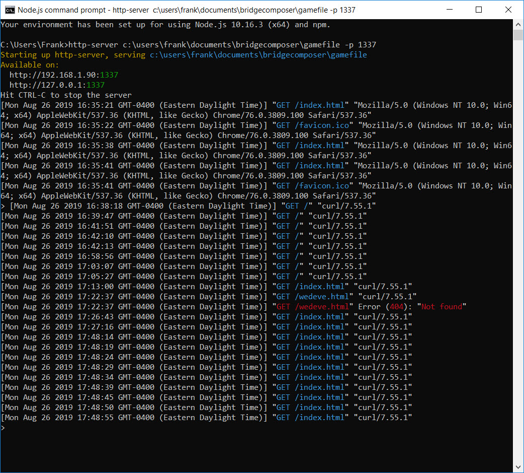
The first log fragment above shows the server starting up, and the first set of http requests. The first half dozen or so requests are from another PC; I did this to initially confirm I could actually reach my localhost server. This first test failed miserably until I figured out I had to disable my PC’s firewall – oops! The next set of lines are from my curl app showing what is actually received by the server when I send a ‘GET’ request from curl.

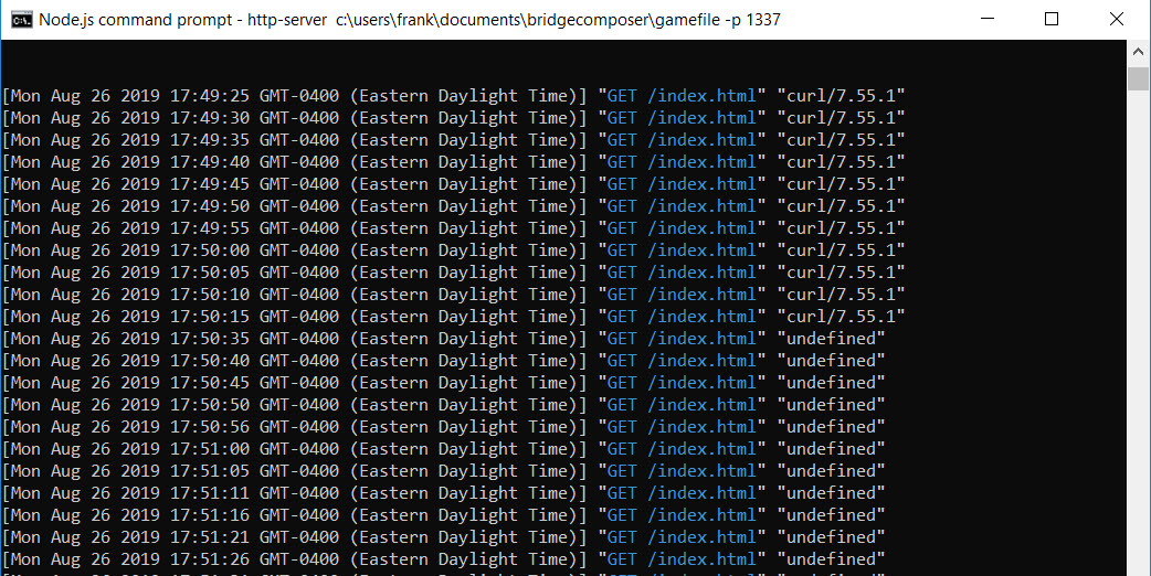
The screenshot above shows some more curl-generated requests, and then a bunch of requests from ‘undefined’. These requests were generated by my ‘WiFiClientBasic’ program running on the ESP32 – success!!

Install ‘curl’

Curl is a wonderful command-line program to generate http (and any other web protocol you can imagine) requests. You can get the executable from this site, and unzip and run it from a command window – no installation required. Using curl, I was able to determine the exact syntax for an http ‘GET’ request to a website, as shown in the screenshot below

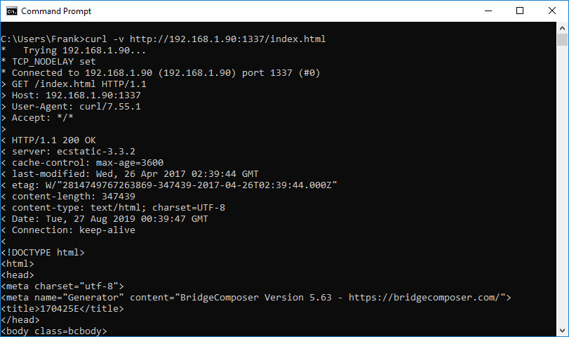
The screenshot above shows curl being used from the command line. The first line C:\Users\Frank>curl -v http://192.168.1.90:1337/index.html generates a ‘GET’ request for the file ‘index.html’ to the site ‘192.168.1.90’ (my localhost server address on the local network), and the -v (verbose) option displays what is actually sent to the server, i.e.

GET /index.html HTTP/1.1
> Host: 192.168.1.90:1337
> User-Agent: curl/7.55.1
> Accept: */*

This was actually a huge revelation to me, as I had no idea that a simple ‘GET’ request was a multi-line deal – wow! Up to this point, I had been trying to use the ‘client.send()’ command in the WiFiClientBasic example program to just send the ‘GET /index.html HTTP/1.1’ string, with a commensurate lack of success – oops!

Modify the WifiClientBasic example program

Armed with the knowledge of the exact syntax required, I was now able to modify the ‘WifiClientBasic’ example program to emit the proper ‘GET’ syntax so that the localhost server would respond appropriately. The final program (minus my network login credentials) is shown below.

/*
 *  This sketch sends a message to a TCP server
 *
 */

//#include <WiFi.h>
#include <WiFiMulti.h>

WiFiMulti WiFiMulti;

char outbuf[100] = { "GET /index.html HTTP/1.1\nHost: 192.168.1.90:1337\nUser-Agent: ESP32\nAccept: */*\n\n" };
//char outbuf[100] = { "GET /index.html HTTP/1.1\n\n" };
char inbuf[200] = { "input buffer" };

void setup()
{
    Serial.begin(115200);
    delay(10);
	Serial.print("outbuf = "); Serial.println(outbuf);
	Serial.print("inbuf = "); Serial.println(inbuf);

    // We start by connecting to a WiFi network
    WiFiMulti.addAP("your_SSID", "your_password");

    Serial.println();
    Serial.println();
    Serial.print("Waiting for WiFi... ");

    while(WiFiMulti.run() != WL_CONNECTED) {
        Serial.print(".");
        delay(500);
    }

    Serial.println("");
    Serial.println("WiFi connected");
    Serial.println("IP address: ");
    Serial.println(WiFi.localIP());

    delay(500);
}

void loop()
{
    const uint16_t port = 1337;
    const char * host = "192.168.1.10"; // ip or dns

    Serial.print("Connecting to ");
    Serial.println(host);

    // Use WiFiClient class to create TCP connections
    WiFiClient client;

    if (!client.connect(host, port)) {
        Serial.println("Connection failed.");
        Serial.println("Waiting 5 seconds before retrying...");
        delay(5000);
        return;
    }

    // This will send a request to the server
	Serial.print("Sending "); Serial.println(outbuf);
	client.println(outbuf);

	int maxloops = 0;
	int numbytes = 0;

	while (!client.available() && maxloops < 1000)
	{
		maxloops++;
		delay(1);
	}
	if (client.available() > 0)
	{
		numbytes = client.readBytes(inbuf, sizeof(inbuf)); // read chars from stream into outbuf
		Serial.print("got "); Serial.print(numbytes); Serial.print(" from server after "); 
		Serial.print(maxloops); Serial.println(" Msec");
		Serial.println(inbuf);
	}
	else
	{
		Serial.print("client.available() returned "); Serial.println(numbytes);
	}


    Serial.println("Closing connection.");
    client.stop();

    Serial.println("Waiting 5 seconds before restarting...");
    delay(5000);
}

* This sketch sends a message to a TCP server

//#include <WiFi.h>

#include <WiFiMulti.h>

WiFiMulti WiFiMulti;

char outbuf[100] = { "GET /index.html HTTP/1.1\nHost: 192.168.1.90:1337\nUser-Agent: ESP32\nAccept: */*\n\n" };

//char outbuf[100] = { "GET /index.html HTTP/1.1\n\n" };

char inbuf[200] = { "input buffer" };

void setup()

{

Serial.begin(115200);

delay(10);

Serial.print("outbuf = "); Serial.println(outbuf);

Serial.print("inbuf = "); Serial.println(inbuf);

// We start by connecting to a WiFi network

WiFiMulti.addAP("your_SSID", "your_password");

Serial.println();

Serial.print("Waiting for WiFi... ");

while(WiFiMulti.run() != WL_CONNECTED) {

Serial.print(".");

delay(500);

}

Serial.println("");

Serial.println("WiFi connected");

Serial.println("IP address: ");

Serial.println(WiFi.localIP());

delay(500);

}

void loop()

{

const uint16_t port = 1337;

const char * host = "192.168.1.10"; // ip or dns

Serial.print("Connecting to ");

Serial.println(host);

// Use WiFiClient class to create TCP connections

WiFiClient client;

if (!client.connect(host, port)) {

Serial.println("Connection failed.");

Serial.println("Waiting 5 seconds before retrying...");

delay(5000);

return;

}

// This will send a request to the server

Serial.print("Sending "); Serial.println(outbuf);

client.println(outbuf);

int maxloops = 0;

int numbytes = 0;

while (!client.available() && maxloops < 1000)

{

maxloops++;

delay(1);

}

if (client.available() > 0)

{

numbytes = client.readBytes(inbuf, sizeof(inbuf)); // read chars from stream into outbuf

Serial.print("got "); Serial.print(numbytes); Serial.print(" from server after ");

Serial.print(maxloops); Serial.println(" Msec");

Serial.println(inbuf);

}

else

{

Serial.print("client.available() returned "); Serial.println(numbytes);

}

Serial.println("Closing connection.");

client.stop();

Serial.println("Waiting 5 seconds before restarting...");

delay(5000);

}

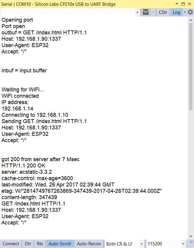
This produced the following output:

Conclusion:

After all was said and done, most of the problems I had getting the ESP32 to connect to the internet and successfully retrieve some contents from a website were due to my almost complete ignorance of HTTP protocol syntax. However, some of the blame must be laid at the foot of the WiFiClientBasic example program, as the lack of any error checking caused multiple ‘Guru Meditation Errors’ (which I believe is Espressif-speak for ‘segmentation fault’) when I was trying to get everything to work. In particular, the original example code assumes the website response will be available immediately after the request and tries to read an invalid buffer, crashing the ESP32. My modified code waits in a 1 Msec delay loop for client.available() to return a non-zero result. As shown in the above output, this usually happens after 5-7 Msec.

In addition, I found that either the full syntax:

GET /index.html HTTP/1.1
Host: 192.168.1.90:1337
User-Agent: ESP32
Accept: */* {newline}

or just

GET /index.html HTTP/1.1{newline}

worked fine to retrieve the contents of ‘index.html’ on the localhost server, because the ‘host’ information is already present in the connection, and the defaults for the remaining two lines are reasonable. However, I believe the trailing {newline} is still required for both cases.

So, now that I can successfully use the ESP32 to connect to my local wireless network and perform internet functions, my plan is to try and use some of the IoT support facilities available on the internet (like Adafruit’s io.adafruit.com) to see if I can get the ESP32 to upload simulated robot telemetry data to a cloud-based data store. If I can pull that off, then I’ll be one step closer to replacing my current HC-05 bluetooth setup (on the 2-motor robot) and/or my Wixel setup (on the 4-motor robot).

Stay tuned!

Frank

Back to the future with Wall-E2. Wall-following Part VI

3 Replies

Posted 13 August 2019

In my last post on this subject, I discussed the idea of using orientation information to compensate raw wall offset distance values to account for the errors associated with robot orientation. The idea was that if I could do that, then Wall-E2 would know how far he was away from the wall regardless of orientation, and would be able to make appropriate corrections to get to and stay at a predetermined offset from the wall.

Well, it didn’t really work out that way. After getting through the geometry analysis and the math, it turned out that in order to use the compensation algorithm, I have to know the initial robot orientation with respect to the wall, and I don’t :-(. Without knowing this, it is basically impossible to apply the correct compensation. For example, if the robot is originally oriented 30º away from the wall, then a ‘toward-wall’ rotation will cause the measured distance to go down, and an upward compensation is required. However, if the robot is initially oriented toward the wall, then that same ‘toward-wall’ rotation will cause the measured distance to go up and a downward compensation is required – bummer!

However, all is not lost; the ability to perform relatively precise angular rotations means that I can use incremental rotations for acquiring and then tracking a predetermined offset distance. In the acquisition phase, the robot orientation is changed in 10º increments in the appropriate direction, and an N-point slope calculation is performed to determine whether or not the current ‘cut angle’ will allow the robot to eventually reach the predetermined offset distance. As the robot approaches the offset line, the cut angle is reduced until it is zero, in theory resulting in the robot travelling parallel to the wall at the offset distance. At this point the robot transitions from ‘capture’ to ‘track’ mode, and the response to distance deviations becomes more robust.

This strategy was implemented using my 2-motor robot, and seems to work well once the normal crop of bugs was eradicated. The following Excel plots show the results of two short runs where the robot first captured and then tracked a 30cm offset setting.

Capture and track a 30cm wall offset starting from the outside

Capture and track a 30cm wall offset starting from the inside

So far I have only implemented this completely for the right side, but as the left side is identical, I anticipate no problems in this regard.

Future Work:

So far I have demonstrated the ability to capture and then track a predetermined wall offset distance, starting from either inside or outside the desired offset distance. This represents a quantum leap in performance, as Wall-E2 currently can only track whatever distance it first measures – it has no capability to capture a desired offset distance. However, there are still some ‘edge’ cases that need to be dealt with one way or the other. For instance, if the robot orientation is too far away from parallel, the current algorithm won’t be able to rotate it enough to capture the desired offset or the measured distance will exceed the max range gate of the ping sensors (currently set at 200cm). These conditions may not be all that deleterious, as eventually Wall-E2 will get close enough to something to trigger an avoidance response, thereby resetting the entire orientation picture (hopefully to something a little more parallel).

In addition to the wall tracking problem, the new capability to make reasonably precise angular rotations should significantly improve Wall-E2’s performance in handling ‘open-corner’ and ‘closed-corner’ situations; currently these cases are handled with timed turns, which are only correct for one floor covering type (hard vs soft) and battery state. With the heading measurement capability, a 90º corner turn will always be (approximately) 90º whether it is on carpet or hard flooring. In addition, now I can program in obstacle avoidance step-turns for approaching obstacles instead of relying entirely the ‘backup-and-turn’ approach.

Stay tuned!

Frank

Back to the future with Wall-E2. Wall-following Part V

08 February 2020 Update:

As I continued my campaign to integrate heading information into my wall-following robot algorithm, my efforts to compensate ‘ping’ distances for off-parallel robot orientations with respect to the nearest wall kept failing, and I didn’t know why. I had gone through the math several times and was convinced it was valid, and as the plot above showed, it should work.

So, I made another run at it, completely redoing the math from the ground up – and running some more test in my ‘local range’ (aka my office). Still no joy – no matter what I did, the math seemed to be overcompensating, as shown in the plot below:

Ping Distance vs Calc Distance for two heading changes

This plot (and others like it) convinced me that I was still missing something fundamental. As I often do, I was thinking about this in bed while drifting off to sleep, and I realized that I might be able to determine the culprit by cheating; I would place the robot at a set distance from the wall, and carefully rotate it manually over a compass rose. At each heading I would manually measure the distance from the ping sensor to the wall, perpendicular to the plane of the sensor (i.e. I would physically measure the distance I would expect the ping sensor to report), and also record the ‘ping’ distance reported by the sensor. With just a few measurements the problem became obvious; the ‘ping’ distance for slant angles to the wall do not even remotely resemble the actual physical distance – it is much less, as shown below.

As can be seen , the compensation algorithm actually works quite well, when dealing with the physically measured slant range. However, because the ‘ping’ distance loses accuracy very rapidly off-parallel angles beyond about 20 degrees, the compensation algorithm is ineffective. A classic case of ‘GIGO’.

After performing the above experiment, I was still left with the mystery of why the compensation algorithm appeared to work so well before – WTF? So, I went back and very carefully examined the previous plot and the underlying data, and discovered I’d made another classic experimental error – The ‘Calculated Distance’ data was plotted on the wrong scale. When plotted on the correct scale, the plot changes to the one shown below:

Previous plot with ‘Calc Distance’ plotted on the correct scale

Now it is clear that the calculated compensation using ‘ping’ distances is not at all useful.

So, the bottom line on all of this it that the effort to apply a heading-based ping distance compensation was doomed to failure from the start, because the distance reported by the ping sensor is wildly inaccurate for off-perpendicular geometries. The good news is that now at least I know why the compensation effort was doomed to fail!

In the meantime, I independently developed a technique for determining the heading required for orienting the robot parallel to the wall as the heading associated with the minimum ping distance achieved by swinging the robot back and forth. This technique utilizes the ping sensors in the realm where they are most accurate, and does away entirely with the need for compensation.

Stay tuned!

Frank

Back to the future with Wall-E2. Wall-following Part IV

When is the robot parallel to the wall?

A unique feature of the point or points where the robot is parallel to the wall is that the ping distance and the calculated distance are equal. However, that’s a bit of ‘chicken and the egg’ as one has to know the robot is parallel in order to use an offset angle of 0 degrees for the compensation calc to work out. Since the heading information available from the MPU6050 IMU is only relative, the heading value for the parallel condition can be anything, and can vary arbitrarily from run to run. So, what to do? One thought would be to have the robot make a short S-turn at the start of any tracking run to establish the heading for which the ping distance goes through a minimum or maximum – the heading for the max/min point would be the parallel heading. From there on, that heading should be reliably constant until the next time the robot’s power is cycled. Of course, a new parallel heading value would be required each and every time Wall-E2’s tracking situation changes (obstacle recovery, step-turns and reversals at the end of a hallway, changing from the left wall to the right one, etc). Maybe a hybrid mode would be feasible, whereby the robot uses uncompensated heading-based S-turns instead of the current ‘bang-bang’ system for initial wall tracking, shifting to a compensation algorithm after a suitable parallel heading is determined.

Looking at the above plots, it may not be all that useful to look for maxima and/or minima, as there are multiple headings for which the ping distance is constant, so which one is the parallel heading? Thinking about ways to rapidly find the parallel heading, it occurred to me that my previous work on quickly finding the mathematical variance of a set of values might be useful here. I plugged the above ping distance numbers into the Excel spreadsheet I used before, and got the following plot of ping distance and 3-element running variance vs time.

So, looking at the above plot, it is encouraging that a 3-point running variance calculation shows near-zero values when the robot is most probably parallel or nearly parallel to the wall. Adding the heading information to the spreadsheet gives the plot shown below

and now it is clear that the large variance values are associated with the changes from one heading to another, and the low variance values are associated with the middle section of each linear heading change (S-turn) segment. If I further enhance the plot by putting the variance plot on a secondary scale and zooming in on the low variance sections, we get the plot shown below:

Variance scale modified to show 0-5 range only

In the above plot, the variance line is zoomed in to the 0-5 range only, emphasizing the 0-0.5 unit variance range. In this plot it can be seen that the variance actually has a distinct minimum very near zero at time points 7, 16, 22, 28-30, and 35-38. These time values correspond to robot heading values of 64, 61, 63, 61-67. and 70-65. Discarding the last set as bad data (this is where the robot literally ‘hit the wall’ at the end of the run), we can compute an approximate parallel heading value as the average of all these values, or the average of 64, 61, 63, 64 (average of 61-67) = 63 degrees. From the video we can see that the robot started out parallel to the wall, and the first heading reading was 62 degrees – a very good match to the calculated parallel heading value.

The next step, I think, is to run some more field tests against a wall, with wall-following and heading assist integrated into the code.

Frank