Tag Archives: IR Follower

IR Modulation Processing Algorithm Development. Part VI

Posted 14 June 2017

In my previous posts on this subject, I have been working with an Arduino Uno as the demodulator processor, but I have been plagued by its limitation of 2KB for program memory. This has caused severe limitations with timing debug, as I can’t make debug arrays long enough for decent time averaging, and I can’t do more than one sensor channel at a time.

So, I finally took the plunge and acquired some of Paul J Stoffregen’s Teensy 3.5 processors from their store.  From their site: “Version 3.5 features a 32 bit 120 MHz ARM Cortex-M4 processor with floating point unit. All digital pins are 5 volt tolerant.” The tech specs are shown on this page, but the main features I was interested in are:

  • 120MHz processor speed vs 16MHz for the Uno
  • 192KB RAM vs 2KB for the Uno
  • Analog input has 13 bit resolution vs 12 for the Uno
  • As an added bonus, the Cortex-M4 has an FPU, so integer-only math may be unnecessary.
  • Much smaller physical footprint – the Teensy 3.5 is about 1/4 the area of the Uno
  • Lower power consumption – The Teensy 3.5 at 120MHz consumes about 30mA at 5V vs about 45mA at 5V for the Uno.

Here are some photos of the Teensy 3.5 as installed on my algorithm test bed, and also on my Wall-E2 robot where it might be installed:

Teensy 3.5 installed on my algorithm test bed, with the Uno shown for size comparison. The small processor in the foreground is an Adafruit ‘Trinket’

Side-by-side comparison of the Uno and Teensy 3.5 SBC’s

Closeup of the Teensy 3.5 shown atop the ‘sunshade’ surrounding the IR sensors.  this is a possible installed location

Wider view of a Teensy 3.5 placed atop the ‘sunshade’ surrounding the IR sensors

In addition to all these goodies, the folks at Visual Micro added the Teensy line to their Microsoft Visual Studio add-on, so programming a Teensy 3.5 is just as easy as programming a Uno – YAY!

Of course, I’ll need to re-run all the timing tests I did before, but being able to create and load (almost) arbitrary-length sample capture arrays for debugging purposes will be a great help, not to mention the ability to use floating-point calculations for better accuracy.

Stay tuned,

Frank


IR Modulation Processing Algorithm Development. Part V

Posted  09 June, 2017

In getting the Arduino code working on my Uno/Trinket test setup (shown below),  I have been having some trouble getting the delays right.  It finally occurred to me that I should run some basic timing experiments, so here goes:

Sample Group Acquisition Loop:

this is the loop that acquires analog samples from the IR detector, and sums 1/4 cycle’s worth into a single ‘sample group’.  To measure this time, I ran the following code:
int startusec = micros();
int sum = 0;
for (int i = 0; i < 1000; i++)
{
int samp = analogRead(SQWAVE_INPUT_PIN1);
sum += samp;
}
int endusec = micros();
Serial.print("time required for 1000 analog read/sum cycles = "); Serial.println(endusec - startusec);

The time required for 1000 cycles was 15064 uSec, meaning that one pass through the loop takes an average of just over 15 uSec. Adding a 85 uSec delay to the loop should result in a loop time of exactly 100 uSec, and a 1000 pass loop time of 100,000 uSec or 0.1sec.  The actual result was 99504, or about 99.5 uSec/cycle – pretty close!

Next, I replaced the summation with a write to a 500-element array (couldn’t do 1000 and still fit within the Uno’s 2K memory limit), and verified that this did not materially change the loop timing.  The time required for 500 loops was 49788; twice that time would be 99576, or almost exactly the same as the 99504 time for the summation version.

Then I tweaked the delay to achieve as close to 25 complete cycles as possible, as shown in the Excel plot below.  With an 82uSec loop delay, the total time for 500 loop iterations was  48272, or about 96.544 uSec per loop iteration.

96.544 uSec per loop iteration, and 20 loop iterations per cycle gives 20*96.544 = 1930.88 uSec per cycle or 518 Hz.  This is very close to the 525Hz value I got from my O’scope frequency readout when I first fabricated my little test setup.

Next, I coded 500 iterations of a two-detector capture/sum operation, and got: “time required for 2-detector 500 analog read/store cycles = 15520”.  So,  about 31 uSec/iteration, or almost exactly twice the one-detector setup.  A four-detector setup yielded a time of  30352 uSec for 500 iterations, or about 60.15 uSec/iteration.  So, a 4-detector setup is possible, assuming the Uno 2KB memory constraint issue can be addressed successfully.

In summary:

  • It takes about 15 uSec to read each sensor’s A/D value and either sum it or store it in an array
  • A four-sensor setup can probably be accommodated, but only if the required summing arrays fit into available memory (not possible for Uno, but maybe for others.
  • A loop delay value of 82 uSec results in almost exactly 20 samples/cycle.

Stay tuned

Frank


IR Modulation Processing Algorithm Development. Part III

Posted 27 May 2017

In my previous post I demonstrated an algorithm for processing a modulated IR signal to extract an intensity value, but the algorithm takes too long (at least on an Arduino Uno) to allow for 20 samples/cycle (admittedly  way over the required Nyquist rate, but…).  So I decided to explore ways of speeding up the algorithm.

First, the baseline:  The starting point is the 17,384  Î¼Sec required to process 100 samples in the current algorithm, or 174 μSec/sample.  At an input frequency of 520Hz,  20 samples/cycle is about 96  Î¼Sec/sample, so I’m off by a factor of 2 or so.  And this is only for  one channel, so I’m really off by a factor of 4 (for a 2-channel setup) or 8 (for my current 4-channel arrangement)

As an experiment, I reduced the running average length from 5 to 1  cycles, or from 100 to 20 samples.  This reduces the shifting operation load by a factor of 5, and resulted in a total processing time of 1876  Î¼Sec  for all 100 samples – wow!

Then I discovered I had failed to uncomment the line that loads the new running average value into the front of the running average array, so I put that back in and re-ran the measurement.  This time the number came up as 10748  Î¼Sec!  This is just not possible!  It is impossible that 10,000 (100 iterations/sample, 100 samples) iterations of a copy operation from one location in the array to another one takes 1/10 the time as 100 iterations (1/sample) of a copy operation from a variable into the array – not possible!!!

But, since it was happening anyway – whether possible or not, I decided I was going to have to figure it out :-(.  So, I changed the line

RunningAvg1[0] = (int)chan1Avg;

to

RunningAvg1[0] = 0;

and re-ran the measurement.  This time the total for processing 100 samples was 1896  Î¼Sec – much more believable!  So, what’s the difference between these two operations?  The only thing I could think of is that it must take a  lot of time to convert a double to an int.

So, I  ran a test where I executed the ‘RunningAvg1[0] = (int)chan1Avg;’ line 10 times, all by itself, and measured the elapsed time.  I got 72  Î¼Sec – a much more believable number, but not what I was expecting.  Increasing the number of iterations to 100 resulted in an elapsed time of 672 μSec – consistent with 72  Î¼Sec for 10 iterations.  That’s nice, but I’m still not any closer to figuring out what’s going on.

Well, after a bunch more experiments, I  think I have the problem narrowed down to the use of floating point math on a few operations.  I have seen some posts to the effect that floating point math is much slower than integer math on Arduino processors, and these experiments tend to bear that out.  I should be OK with integer math everywhere, I hope ;-).

After completely re-writing the algorithm to eliminate floating point math (and correcting several logic errors – oops!), I re-ran the 100-element process for 1 channel, with the following results:

All components – original captured samples, running average, AC component, and full-wave rectified component. Note elapsed time of 3008 uSec

From the above Excel plot, it is clear that the algorithm successfully  extracted the full-wave rectified value for the incoming modulated IR signal, and did so in only 3008 uSec for 100 samples.  This should mean that I can easily handle up to three simultaneous channels, and maybe even four – YAY!

Another run with two simultaneous channels  was made.  The following Excel plot shows the Channel 2 results, along with the elapsed time for both channels.

Channel 2 all components – original captured samples, running average, AC component, and full-wave rectified component. Note elapsed time of 4268 uSec

The above results for two channels strongly suggests that all four channels in the current hardware implementation can be processed simultaneously while still maintaining a 20 sample/cycle sample rate.  This is extremely good news, as it implies that I can ‘simply’ insert an Arduino Uno or equivalent between the detector array and the robot controller.  The robot contoller will continue to see left/right analog values as before (but inverted – more positive is more signal), but background IR interference will be averaged out by the intermediate processor – cool!

Rather than use a Uno, which is physically very large, I hope to be able to use something like an Adafruit Arduino Pro Micro, as shown below:

Adafruit’s Arduino Pro Micro. 16MHz, 9 Analog 12 Digital I/O

This should fit just about anywhere (probably on top of the sunshade), and be very easy to integrate into the system – we’ll see.

Stay tuned!

Frank


IR Modulation Processing Algorithm Development. Part II

Posted 25 May 2017

One of the things I didn’t understand about the analog sample runs from my previous post  was why there were so many cycles of the IR modulation signal in the capture record; I had set the algorithm up to capture only 5 cycles, and there were more than 10 in the record – what gives?

Well, after a bit of on-line sleuthing, I discovered the reason was that the A/D conversion process associated with the analogRead() function takes a  LOT longer than a digitalRead() operation.   This put a severe dent in my aspirations for real-time processing of the modulated IR signal, as I would have to do this for at least two, and maybe four independent signal  streams, in real time – oops!

One thing I have discovered for sure in the modern internet era; if you are having a problem with something, it is a certainty (i.e. Prob = 100%) that many others  in the universe have had the same problem, and most likely someone has come up with (and posted about) one or more solutions.  So, I googled ‘Arduino Uno  faster  analogRead()’, and got the following hits:

The very first link above took me to this forum post, and thanks to jmknapp and oracle, I found the Arduino code to reset the ADC clock prescale factor from 128 to 16, thereby decreasing the conversion time by a factor of 8, with no reduction in ADC resolution – neat!

To test the effect of the prescaler adjustment, I measured the time it took for 100 ADC measurements with no delay between measurements.  As shown below, there is a dramatic difference in the ‘before’ and ‘after’ plots:


100 ADC cycles with no delay, prescale = 128

100 ADC cycles with no delay, prescale = 16

Next, I adjusted the delay between ADC cycles to collect approximately 5 cycles at the 520Hz input rate, as shown below:

Delay adjusted so that 100 samples ~ 5 cycles at 520Hz.

With the prescaler set to 16, the ADC is  much faster.  With a 5-cycle collection window at 520Hz, I have 80 uSec/cycle to play with for other purposes, so it seems reasonable that I can handle multiple input streams with relative ease – YAY!!.

The next step was to simulate a 4-channel capture operation by capturing 400 samples, 100 each from four different channels. In this simulation, all the data comes from the same IR link, but the processing load and timing is the same.  All the samples from the same time slot are taken within a few microseconds of each other, and the loop (inter-sample) delay was adjusted such that approximately five cycles were captured from each ‘channel’, as shown in the following Excel plot

Simulated 4-channel capture

As can be seen in the above plot, the channel plots overlap almost exactly.  What this shows is that the Arduino Uno can capture all four IR detector channels at sufficient time resolution (about 20 samples/cycle) for effective IR signal detection/evaluation, and with sufficient time left over (about 30 uSec) for some additional processing.

If the design is changed from four channels to just two, then the processing load goes down significantly,  as shown in the following plot

Simulated 2-channel capture

To complete the simulation, I added the code to perform the following operations on a sample-by-sample basis:

  • Update  the running average of the sample array
  • Subtract the running average from  the sample, and take the absolute value of the remainder (full-wave rectification)
  • Store the result in another array so it can be plotted. This last step isn’t necessary except for debugging/evaluation purposes

Initial results as shown below are very promising. The following Excel plots show the results of processing 100 ADC samples in real time.  First 100 samples were loaded into an array to represent the last 100 samples in a real-time scenario, and the running average value was initialized to the average of all these samples.  Then each subsequent real-time sample was processed using the above algorithm and the results were placed in holding arrays for later printout, with the following results

All components – original captured samples, running average, AC component, and full-wave rectified component

Detail view of original captured samples and the running average component

Detail view of the AC component of the original captured samples and the computed full-wave rectifed component

The above plots confirm that the ADC samples can indeed be processed to yield the full-wave rectified intensity of a modulated IR beam.  However, there is a fly in the ointment – it takes too long; it took 17,384  Î¼Sec to process 100 samples – but 100 samples at 20 samples/cycle only takes approximately 9600  Î¼Sec – and this is only for one channel :-(.  I will need to find some serious speedup tricks, or reduce the number of samples/cycle, or both in order to fit the processing steps into the time available.

Stay tuned,

Frank


IR Modulation Processing Algorithm Development – Part I

Posted 23 May 2017

As you may recall from previous posts, I have been collaborating with my long-time friend and mentor John Jenkins on the  idea to use square-wave modulation of the charging station IR beam to suppress ‘flooding’ from ambient IR sources such as overhead incandescent lighting and/or sunlight.

More than likely, If it is possible to implement a software processing algorithms to recover steering information from potentially corrupted data, it will have to be housed on a dedicated processor.  So, I decided to set up a separate test setup using two processors – one to generate a square-wave modulation waveform, and another to receive that waveform through an IR link.  The link can then be modified in a controlled way to simulate link losses and/or ‘flooding’.  The initial hardware setup is shown below.

Initial test bed verification using 12cm separation

Scope shot showing transmitted and received waveforms, 12cm separation

Algorithm test bed with IR link range set to 78cm

Then I ran my little test program on the receiver processor that simply acquires 100 samples at roughly 20 samples/cycle and then prints out the results.  The following two images are Excel plots of the results for 12cm & 78cm separation.

As can be seen from these two plots, the 12 & 78cm separation values provide a reasonably good simulation of the ‘very good’ and ‘reasonably crappy’ signal conditions.

Next I verified that I can successfully ‘flood’ the receiver with my portable battery-operated IR signal generator.  I monitored the transmitted  and received waveforms, without and then with flooding.  In both cases, the  bottom trace is the 5V square-wave transmitted signal, shown at 2V/div, and the top trace is the received signal shown at 1V/div.  The ground for both traces is the same line on the scope screen.

78cm separation, no flooding signal. Bottom trace is transmit @ 2V/cm, top is receive @ 1V/cm, ground for both is same line

78cm separation, with flooding signal. Bottom trace is transmit @ 2V/cm, top is receive @ 1V/cm, ground for both is same line

Applying flooding signal with battery-operated IR signal generator

As can be seen in the scope photos, I can indeed produce almost 2V of ‘flooding’ using the IR signal generator, so I should be able to determine whether or not a particular recovery algorithm is successful at suppressing flooding effects.

Stay tuned

Frank


Charging Station System Integration. New Sunshade Testing

Posted 19 May 2017

While working with John Jenkins on the modulated IR beam idea, I decided to run some tests with the current 4-detector design, to see how the new sunshade with center divider was affected by  ambient IR on a bright sunny day.  So, I disabled Wall-E2’s motors and then placed it at several different critical spots in the entry hallway.  At each location I used my little IR test generator to mark the beginning and the end of the test for that location, and then moved on to the  next one.  The locations are shown in the following photos, in the order that the tests were run.

Position 1: Near where Wall-E2 transitions from wall-tracking to IR beam homing

Position 2: This is where Wall-E2 has been winding up when it homes on the outside sunlight instead of the IR beam

Position 3: Here Wall-E2 should be firmly fixated on the IR beam

These results, combined with my earlier IR response tests with a single phototransistor are encouraging, because it is clear that at least in this case, Wall-E2 should have no difficulty discriminating between the ambient IR and the charging station IR beam.

I ran some homing tests, which Wall-E2 handled with ease; unfortunately God had already turned the lights out on this side of the world, so the tests weren’t in the presence of daylight IR interference.  I’ll do some more real-world discrimination testing tomorrow, and  I am  hopeful that the new sunshade-with-divider version will be successful, at least for this part of the house.

Stay tuned,

Frank


IR Light Follower for Wall-E2, Part XI. Center Divider Investigation

Posted 16 May 2017

One of the suggestions John Jenkins made during his visit, in addition to the idea of modulating the IR beam to suppress ‘flooding’ from ambient IR sources, was the idea of placing an opaque divider between the left and right halves of the detector array.  He thought that I might even be able to reduced the detector array from four to two phototransistors and still get good homing performance, assuming that each of the two detectors had sufficiently wide beamwidths to accommodate off-axis IR beam intercepts.  The current detectors have a +/- 12 º beamwidth, but are arrayed in such a way as to provide well over 60 º aggregate coverage.  To do the same thing with just two detectors would require parts with considerably wider beamwidths.  the TAOS TSL267 (another one of JJ’s suggestions) has an approximately +/-30 º beamwidth at the half-response points, so they seem almost ideally suited for  this application.  As a major added bonus, the TAOS parts feature a photo-diode integrated with an op-amp to address the dynamic range issue mentioned by John.  The diode operates in its linear range, and the op-amp amplifies the IR signal to useful levels.  The only fly in the ointment is that the op-amp gain isn’t adjustable, and its output limits at fairly low light levels – bummer!

Loader Loading...
EAD Logo Taking too long?

Reload Reload document
| Open Open in new tab

Download

In order to investigate  the opaque divider idea, I decided to run some bench angular response tests using my robot’s 4-detector array with and without a center divider.  I printed out a copy of the compass rose graphic I had hanging around from my magnetometer project (one of my more spectacular failures) and set up a bench test with Wall-E2 and my little IR test source, as shown below.

Angular response test setup

Closeup of the ‘sunshade’ cowling (black rectangular opening) around the 4-detector array

Closeup of sunshade with divider installed

The results without the center divider were about as expected, with about +/- 45 º coverage, as shown in the Excel plot below

Response vs angle for 4-detector array, without center divider

+/- 60 deg response vs angle for 4-detector array, without center divider

With the divider, the response appears to be about the same (note here that the ‘with divider’ response is flipped left/right from the ‘no divider’ case – oops!)

+/- 30 deg response vs angle for 4-detector array, without center divider

Note in the above ‘detail’ view that the response curves for the two center detectors (DET2 & DET3) seem to be very symmetric about the 0 º point, as expected.  What this also shows is that just these two detectors could probably be used for homing, if off-axis beam detection weren’t a consideration.

+/- 30 deg response vs angle for 4-detector array, with center divider

The ‘with divider’ plot above shows a significant difference from the ‘no divider’ plot, right at the center.  In the ‘no divider case, the DET1 & DET2 responses are very nearly the same, but in the ‘with divider’ case they are significantly different, and almost perfectly anti-symmetric about the center.  This  should allow more precise detection of small left/right deviations from the beam centerline, and therefore more precise homing.

Stay tuned!

Frank


IR Phototransistor Sensitivity/Dynamic Range Study

Posted 05/14/17

In a previous post, I mentioned that John Jenkins, mentor and old friend, had  some ideas regarding my Wall-E2 robot’s problems with homing in on an  IR beam in the presence of ambient IR sources like overhead incandescent lighting and/or sunlight streaming in through windows and doors.   John pointed out that this was really a system dynamic range issue, and it was likely that, as currently configured, the IR phototransistors were running out of dynamic range (saturating) well before the 10-bit A/D’s on the AtMega SBC.  In order to get the detector sensitivity up to the  point where Wall-E2 could ‘see’ the IR beam far enough (1.5-2m) away to avoid hanging up on the lead-in rails (see this post  and this post for details), I had to use a very high value collector resistor (330K), which reduces the dynamic range significantly.

In a subsequent email conversation, John suggested that the proper way to handle this problem was to reduce the collector resistor to the point where the detector doesn’t saturate under the worst case ambient IR conditions, and then add amplification as necessary  after the detector stage to get the required sensitivity.  John’s point was that as long as the detector response is relatively linear (i.e., it’s not saturated), then there shouldn’t be any loss of information through the stage, so a later linear amplification stage will allow the desired IR signal to be detected/processed even in the presence of interference.  However, if the detector stage saturates due to interference, then it’s basically ‘game-over’ in terms of the ability to later pull the desired signal out of the noise.

This wasn’t exactly what I wanted to hear, as adding the required post-detector amplification stage wasn’t going to be particularly easy – there’s not much left in the way of free real-estate on Wall-E2’s main platform (there’s plenty of room on the second level, but putting stuff there requires inter-level cabling and is a major PITA).  As I was thinking this, I had a flashback to similar conversations with John from 40-45 years ago, when we were both design engineers in a USG design lab; the usual outcome of such ‘conversations’ (to the uninitiated these might be mistaken for shouting matches) was that my circuit got ‘simplified’ by the addition of 50% more parts – but could then withstand a nuclear attack in the middle of a snowstorm at the South Pole!

Anyway, back in the present, John suggested I run some experiments designed to determine the ratio of IR field intensity to collector current for a the  phototransistors I was using, so the proper collector resistor value to be computed to utilize the available detector dynamic range without driving it into saturation.  His suggestion was to not  use a collector resistor at all, but to simply connect the collector to +VDC through a current meter, and then expose the detector to worst-case ambient conditions.  I didn’t particularly like this idea, because I only have a manual non-recording multimeter, and I wanted to record the data for later analysis.  So, I decided to program up one of my small SBC’s with analog input capability (in this case, a Pololu Wixel), and set up to measure the voltage drop across  a 10  Î© precision resistor in the collector circuit.  The hardware setup is shown in the following photo

Hardware setup for IR Phototransistor Response Experiment

Before and after collecting ‘field’ data, I made a collection run on the bench, using my IR LED test box, with the following results.  As can be seen in the plot, the maximum voltage drop across the 10Ω resistor was approximately 200mV, or about 20mA.

IR detector response bench test. Nose-to-nose with my IR test source

Bench test with IR LED test generator


To collect the ‘field’ data, I placed the SBC in different locations around the house, and recorded A/D values.  For these experiments I was using an example Wixel app that printed out the A/D values for all 6 analog inputs, scaled such that the maximum reading was equivalent to the SBC board voltage (3.3V) in millivolts.  In other words, the maximum A/D reading was approximately 3375, or about 3 mV/bit

Location 1: Looking out glass doors on south side of house

Location 2: Direct sunlight through window on south side of house

Location 3: Kitchen floor, looking toward entrance hall and atrium

Location 4: Entry hallway, looking toward atrium. This is the usual starting location for charging station homing tests

Location 5: Entry hallway near door to atrium

These results were not at all what I expected.  Either there is something wrong with the experimental setup, or the ambient light IR field intensity isn’t anywhere near as  strong as expected.  If the data can be believed, the ambient conditions are significantly weaker than the bench-test conditions, which were basically nose-to-nose with my IR test LED.  So, if my planned  double-check of the hardware doesn’t find any problems, then I’ll change the resistor value from 10Ω to 100Ω and repeat the tests.

17 May 2017 Update

After thoroughly reviewing the hardware setup, I concluded that everything was working properly, but that the 10Ω load resistor simply didn’t provide sufficient drop for reliable measurements.  So, I changed out the 10Ω resistor for 100Ω, and repeated the tests, with the following changes:

  • As before, I started the run by performing a ‘nose-to-nose’ test to verify proper operation, but this time I measured the detector current using a multimeter. The  result was about 15mA maximum current.
  • At each of the 5 locations, I started with a short nose-to-nose section (not shown in the plots) to make sure the detector was operating properly
  • At location 2 (the direct sunlight location), I physically oriented the detector for maximum response.
  • After location 5, I placed the detector on the charging station’s IR beam reflector boresight at about 0.5m distance, and physically oriented the detector for max response.
  • I calculated the detector current for each reading, and plotted that rather than the raw reading.  To calculate the detector current for each measurement, I subtracted the  detector reading from the corresponding 3.3VDC supply  voltage measurement and divided by 100.

The results of these tests are shown in the plots below:


These results are pretty interesting.  As I’m sure John would point out, the direct sunlight response of about 0.2 mA is about 20 times the value required to saturate the phototransistor with  the current 330KΩ.  No wonder I was having interference problems – oops!

Stay tuned!

Frank


Charging Station Design, Part XIV – Modulated IR Beam Study

Posted May 10, 2017

A couple of weeks ago my old friend and mentor John Jenkins was visiting the area and stopped in for a couple of days.  Naturally I had to show him my Wall-E2 robot, complete with autonomous charging capability.  Just as naturally (if you believe in Murphy’s law), Wall-E2 refused to cooperate.  Instead of homing in on the charging station, it blissfully homed in on the sunlight streaming in through the atrium, bypassing the charging station entirely!

After John got through laughing, he mentioned that he knew of some other IR-following robotics projects where the designers used a modulated IR beam to allow the robot to discriminate between general IR background noise and the intended signal.  So, I decided to start a feasibility study to see if I could incorporate some sort of modulation into the design of the charging station, without completely overtaxing either the charging station, or the robot, or both!

I started with the idea that I could easily add square wave modulation to the IR beam by simply switching the LED off & on at some reasonable rate (say, 500Hz).  The problem occurs on the other end (the robot), as it will somehow have to a) detect the square wave signal, and b) still have the ability to home in on the modulated signal – i.e. still be able to determine  signal variation across the four photo-transistor  array.

To investigate,  I created a square wave generator using an Adafruit Trinket, and a square wave receiver using an Arduino Uno, as shown in the following photo

Adafruit Trinket SBC used for generating the square wave signal, and an Arduino UNO used as the receiver

Square wave signal from the Trinket

The first step was to see if the Arduino Uno was fast enough to accurately detect the square wave pattern, so I simply grabbed 100 samples from the input pin using digitalRead() with a delay of about 1/10 of the waveform period.  Then I plotted the data in Excel, as shown below:

Digital samples from Arduino Uno ‘receiver’

As can be seen from the plot, there are plenty of samples per cycle, well above the Nyquist rate for the dominant signal term.

Next, I moved the square wave signal to an analog input on the Uno, and reprogrammed to collect analog values vice digital ones, as shown below:

Analog readings with 500Hz square wave input

As can be seen,  the analogRead() function is plenty  fast enough to accurately reproduce the digital square wave signal, with about 10-13 samples/cycle.  So, at least in principle I should be able to detect a square-wave-modulated IR beam, and determine its ‘field strength’ (analog reading when the beam is ON) for homing purposes.

Stay tuned!

Frank


Charging Station System Integration. Part III

Posted 15  April 2017

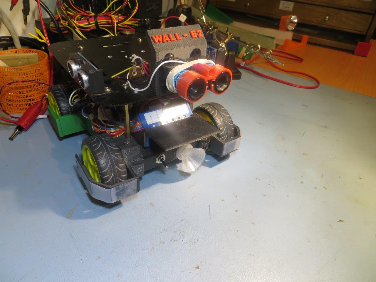
In my previous post on this subject, I described some IR homing tests with and without the overhead incandescent lights, and  the development of a ‘sunshade’ to block out enough of the IR energy from the overhead lamps to allow Wall-E2 to successfully home in on the IR beam from the charging station.  At the conclusion of that post, I had made a couple of successful runs using a temporary cardboard sunshade, and thought that a permanent sunshade would be all that I needed.

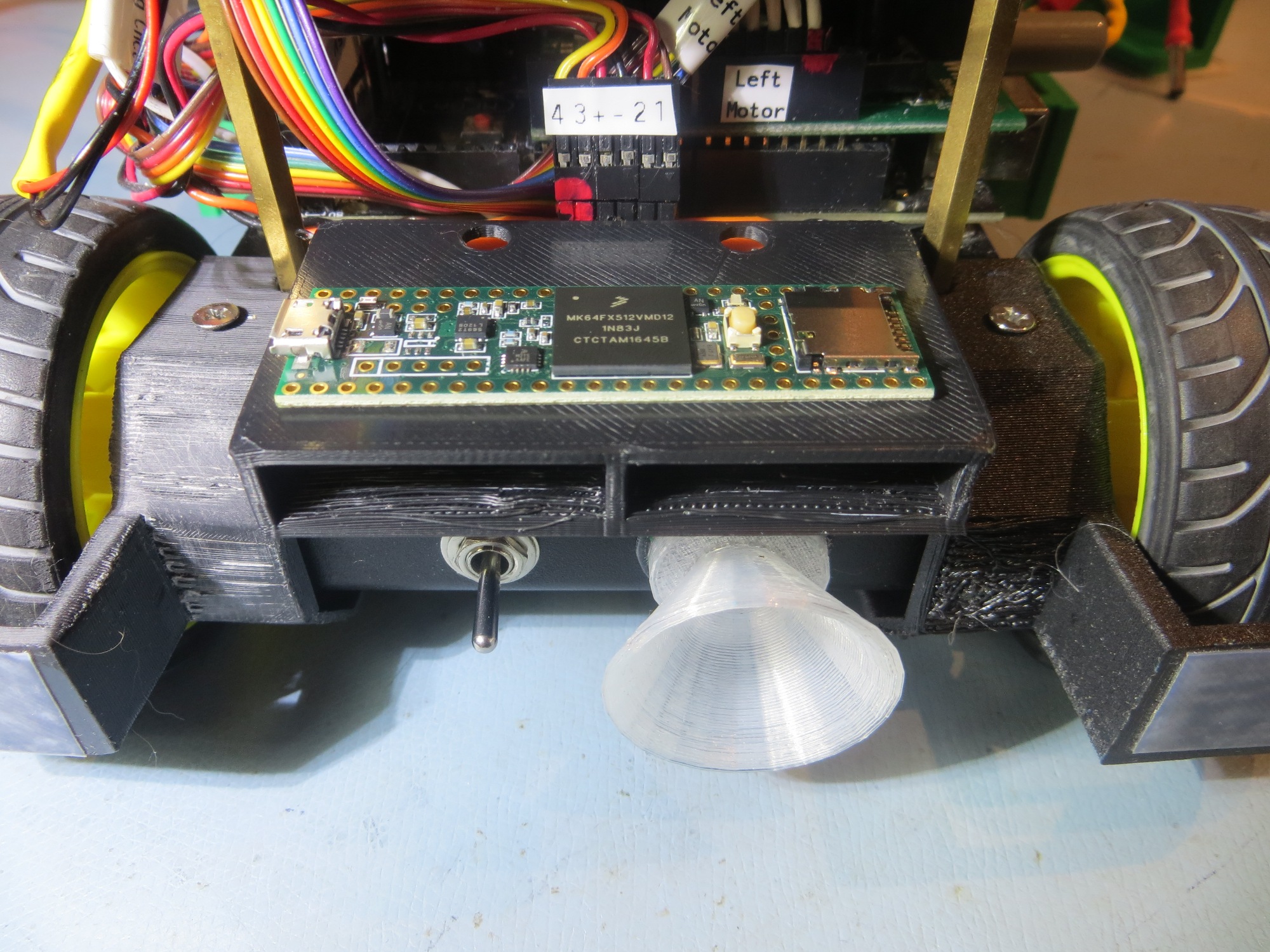
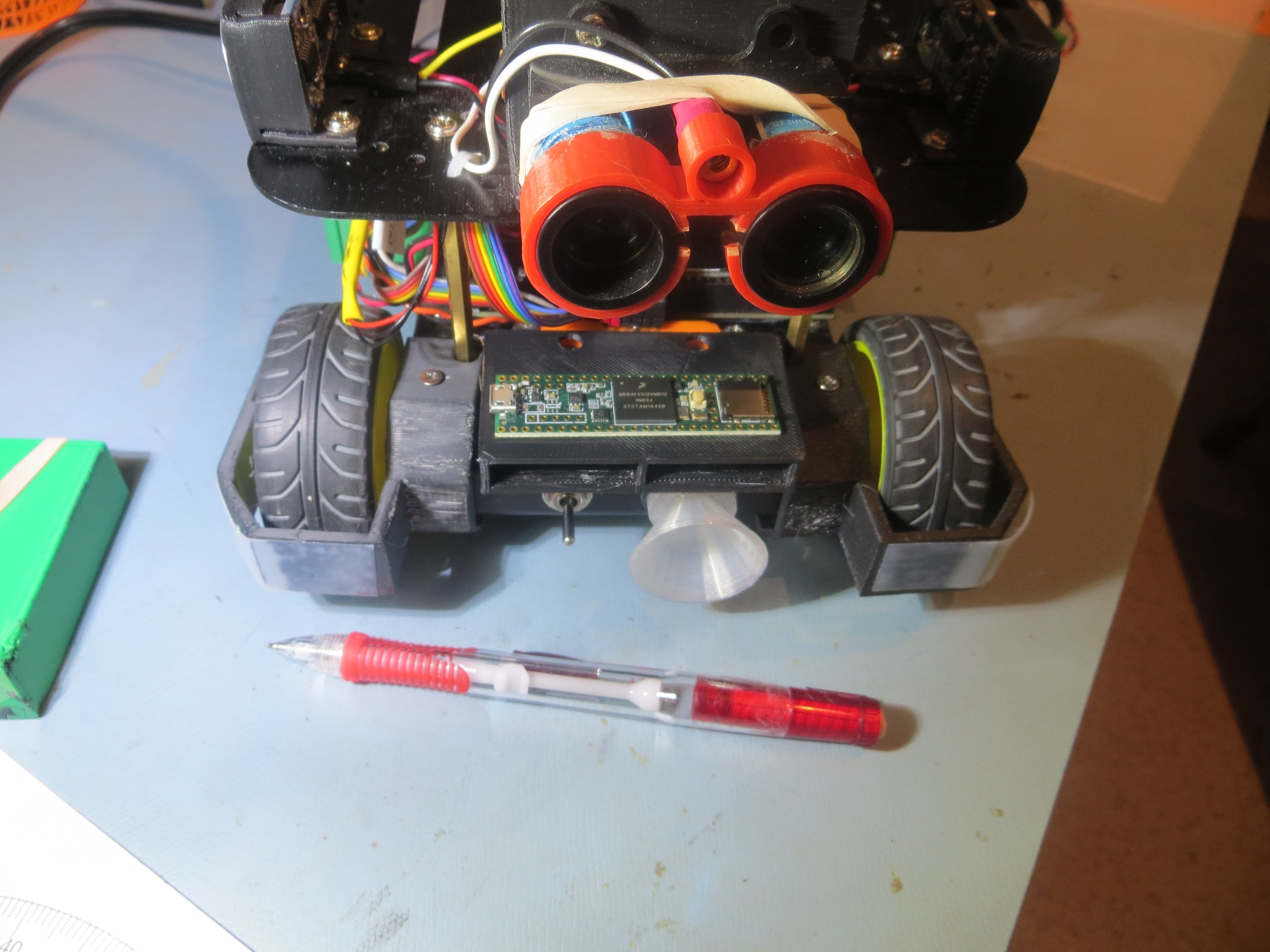
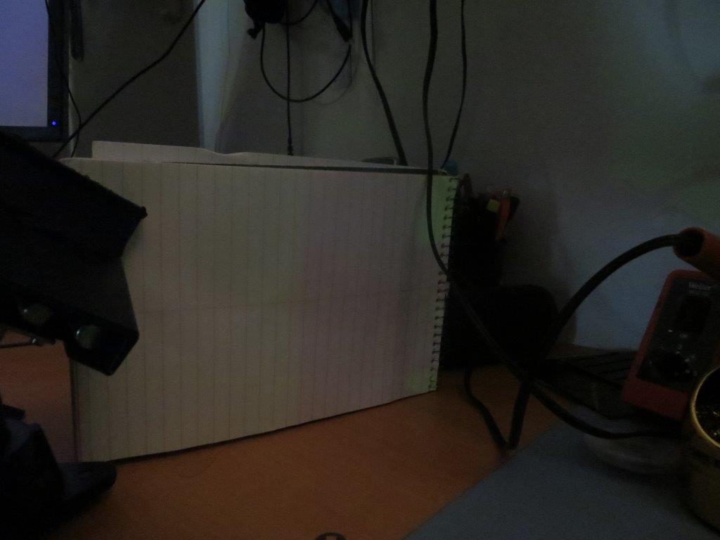
However, after installing the sunshade (shown below), I discovered that the homing performance in the presence of overhead IR lamps was marginal when the robot’s offset distance from the wall was more than about 50 cm.

Sunshade, oblique view
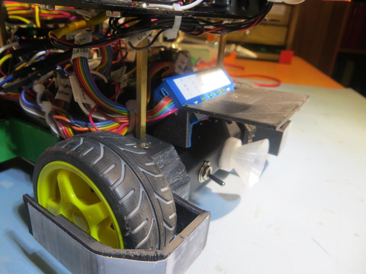
Sunshade, side view

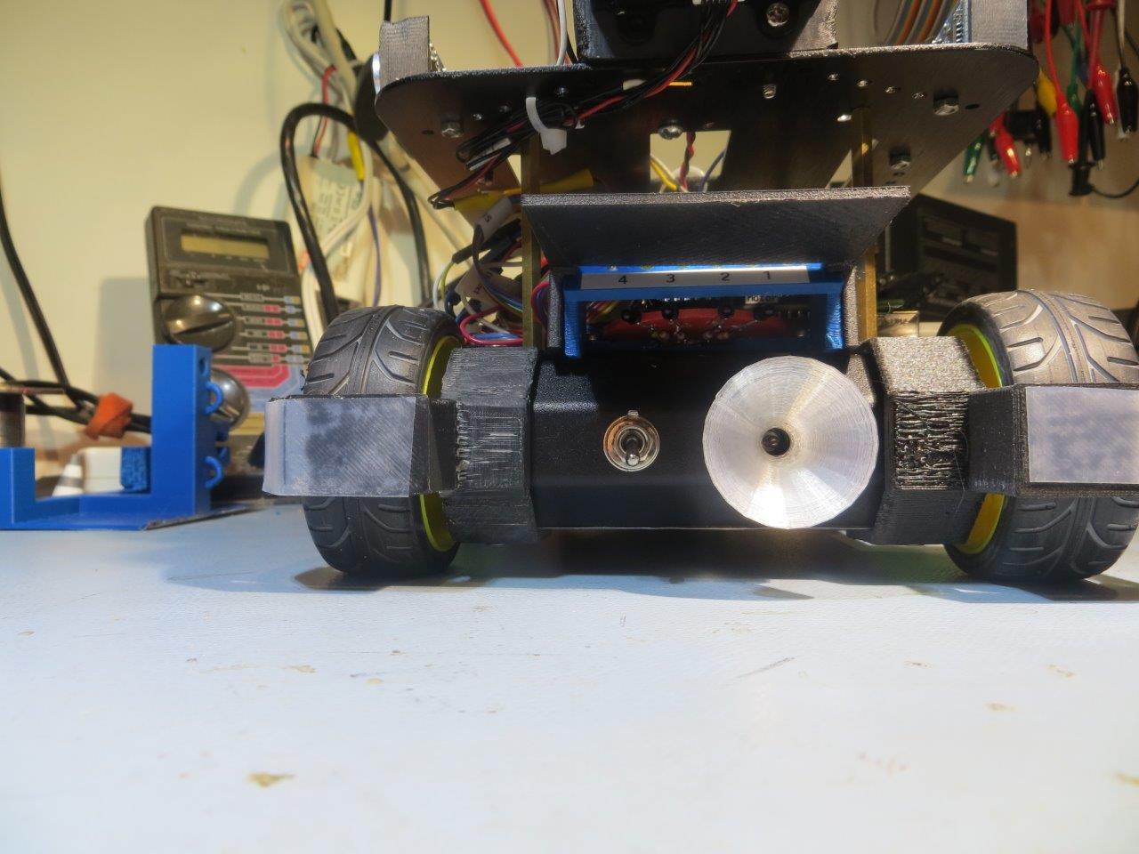
Sunshade, front view

Apparently  the IR interference was causing the robot to not respond to the IR beam until too close to miss the outer lead-in rail.  This issue was explored in an earlier post, but I have repeated the relevant drawings here as well.


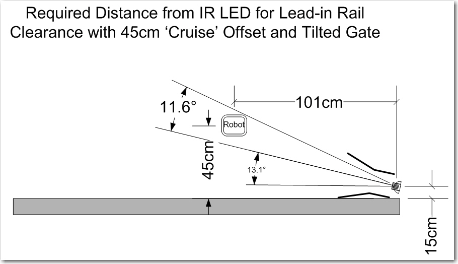
Tilted gate option. The tilt decreases the minimum required IR beam capture distance from about 1.7m to about 1.0m

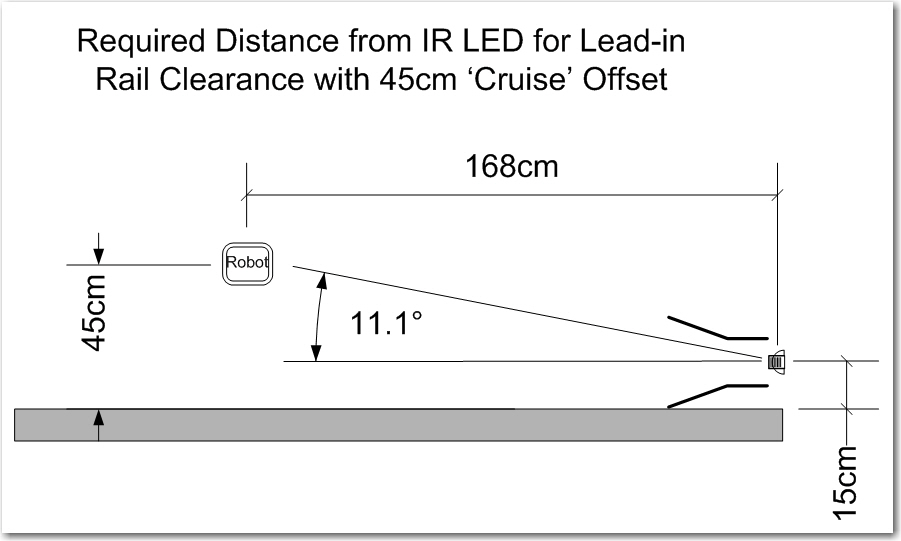
Capture parameters for the robot approaching a charging station

When the robot is ‘cruising’ at more than about 50 cm from the tracked wall,  the IR interference from the overhead lamps prevents the robot from acquiring the charging station IR beam until too late to avoid the outer lead-in rail, even in the 13 º tilted rail arrangement in the first drawing above.


So, what to do?  I am already running the IR LED at close to the upper limit of the normal operating current, so I can’t significantly increase the IR beam intensity – at least not directly.  I can’t really increase the size of the ‘sunshade’ dramatically without also significantly affecting the IR beam detection performance.  What I really needed was a way of increasing the IR beam intensity  without increasing the LED current.  As it turns out, I spent over a decade as a research scientist at The Ohio State University ElectroScience Lab, where I helped design reflector antenna systems for spacecraft.  Spacecraft are power and weight limited, so anything that can be done to improve link margins without increasing weight and/or power is a  good thing, and it turns out you can do just that by using  well-designed reflector dishes to focus the microwave communications energy much like a flashlight. You get more power where you want it, but you don’t have to pay for it with more power input; the only ‘cost’ is the insignificant added weight of the reflector structure itself – almost free!  In any case, I needed something similar for my design, and I happened to have a small flashlight reflector hanging around from a previous project – maybe I could use that to focus and narrow the IR beam along the charging station centerline.

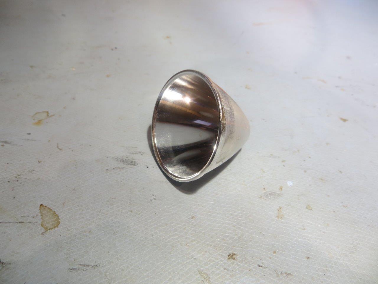
LED flashlight reflector

So, using my trusty PowerSpec PRO 3D printer and TinkerCad, I whipped up an experimental holder for the above reflector, as shown below

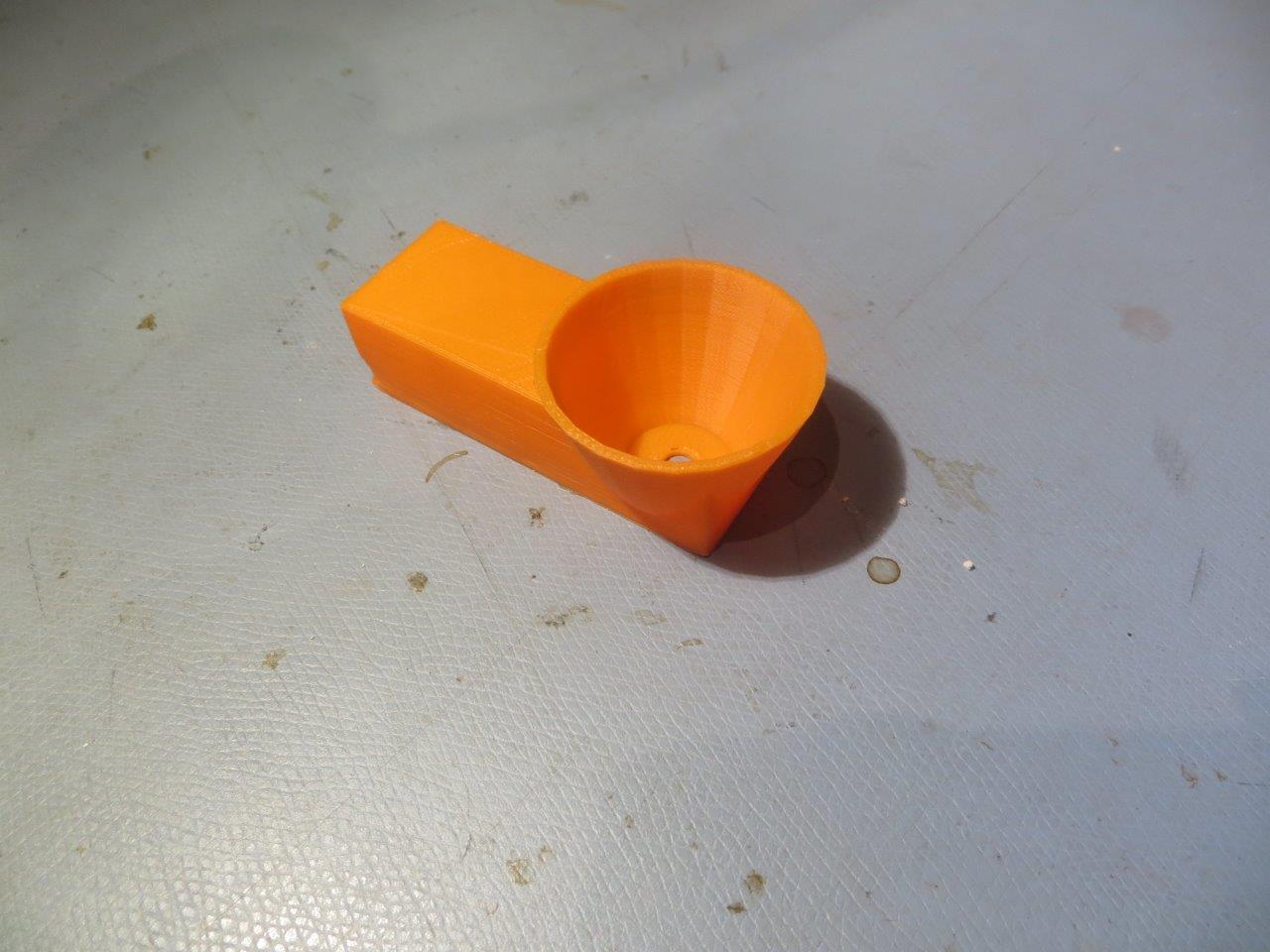
Experimental 3D-printed flashlight reflector holder

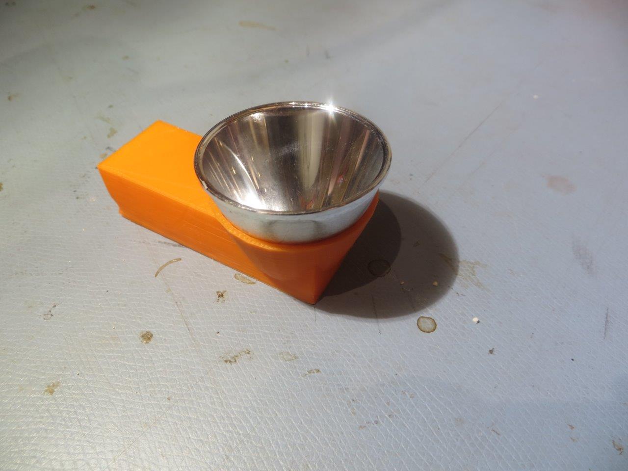
Reflector mounted on experimental holder

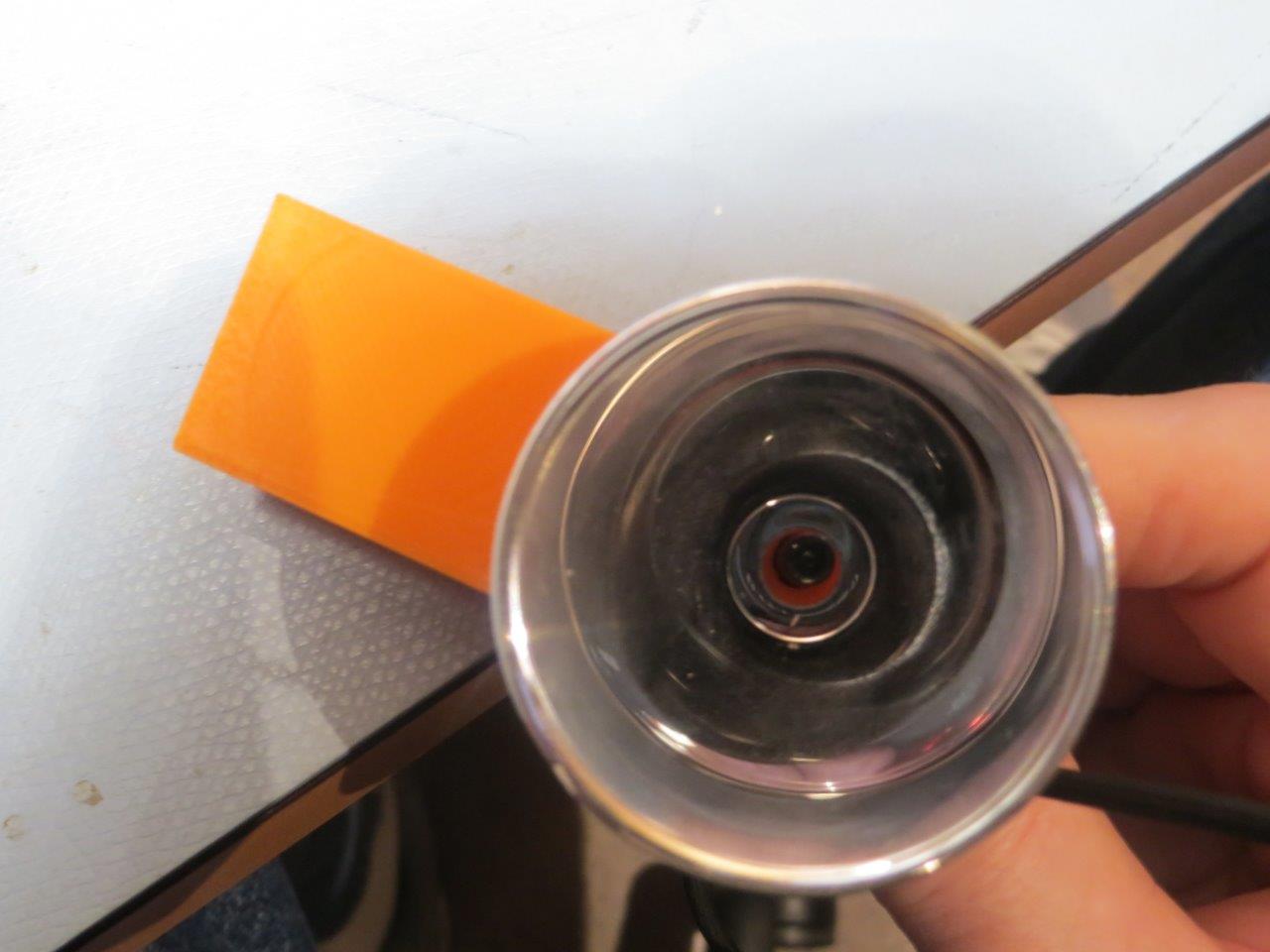
IR LED mounted on reflector

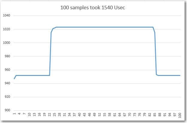
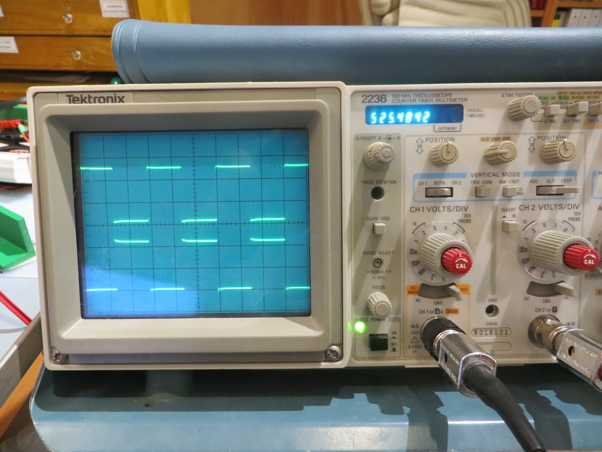
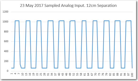
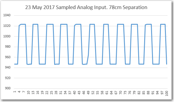
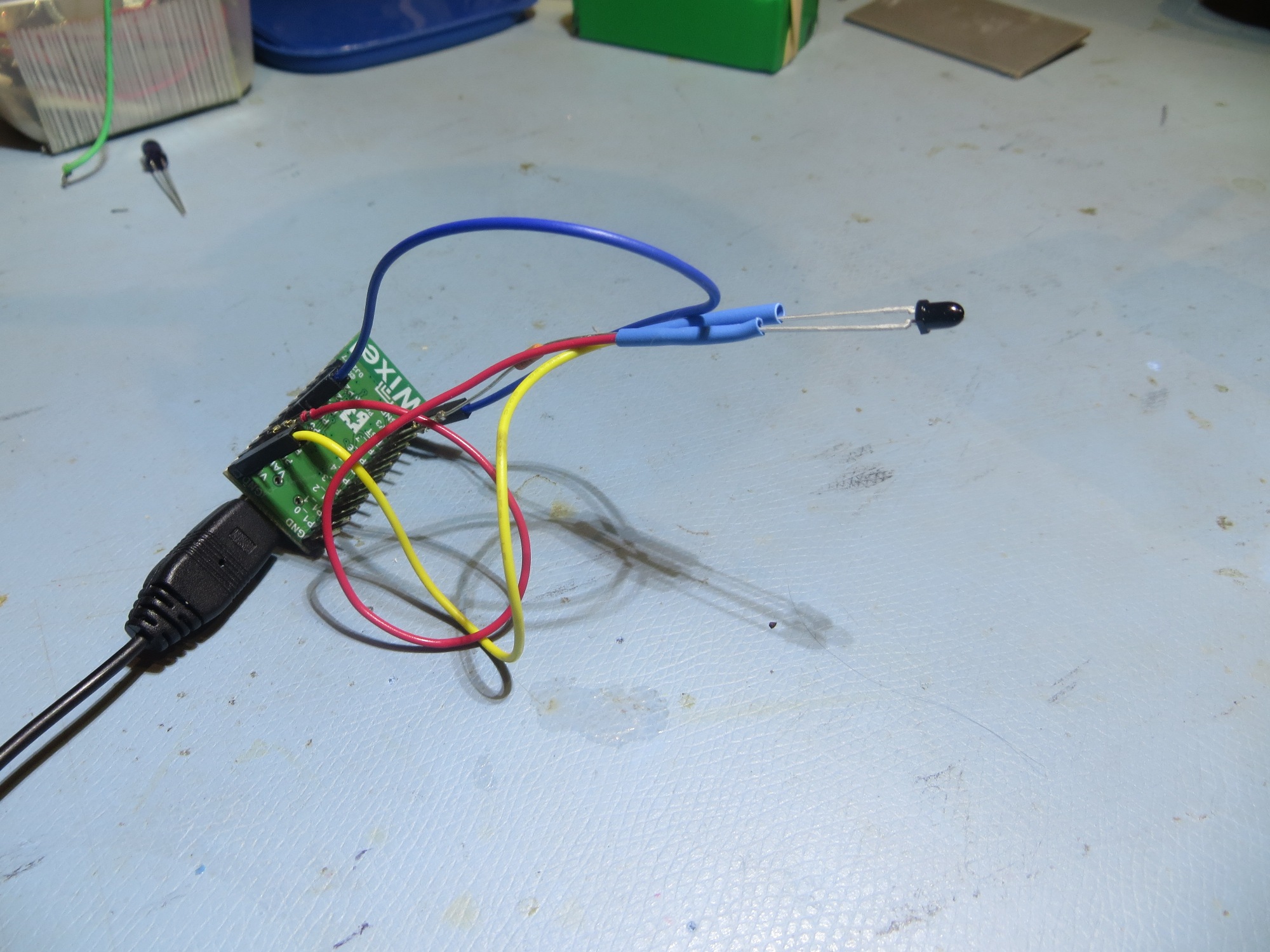
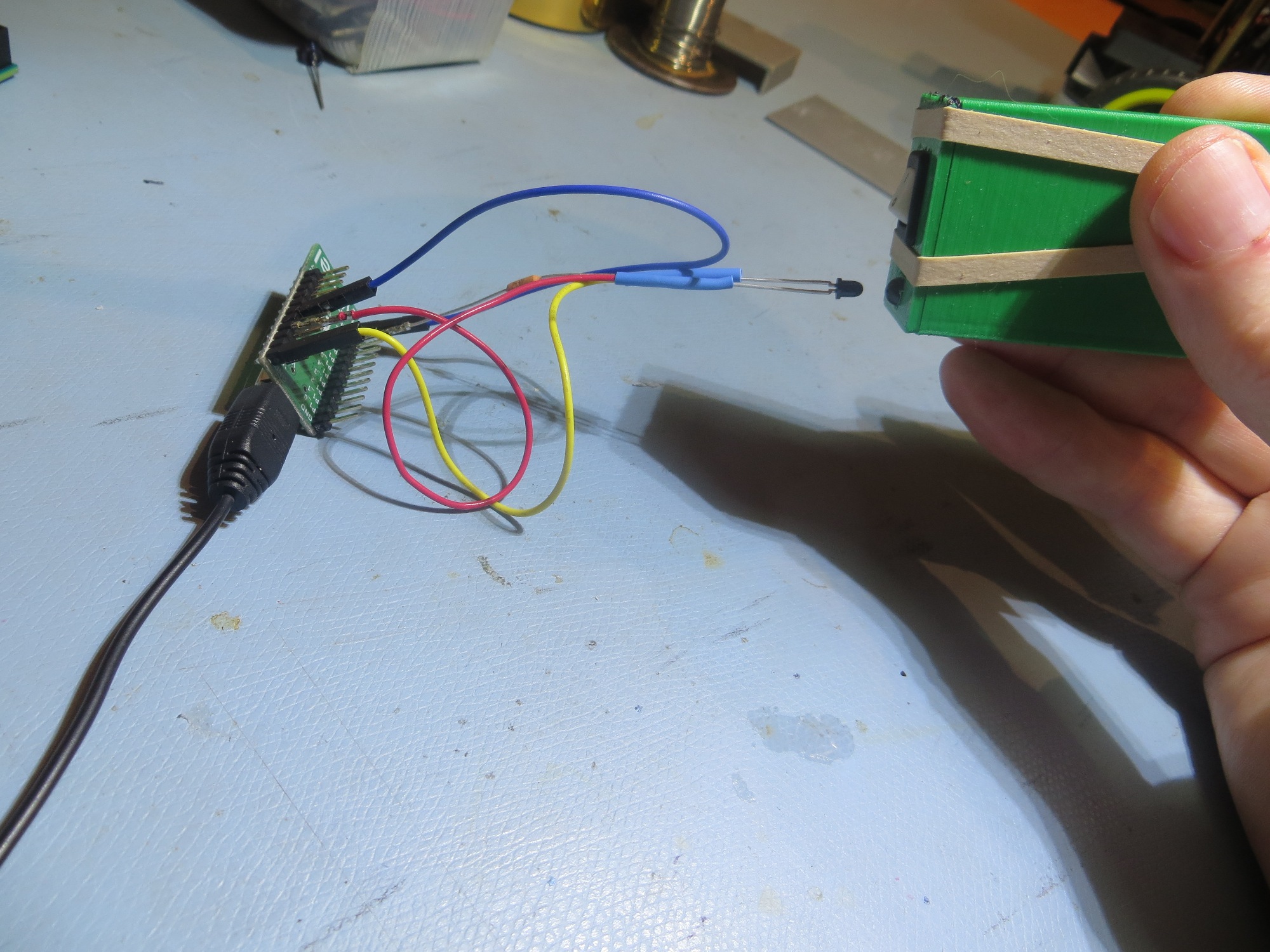
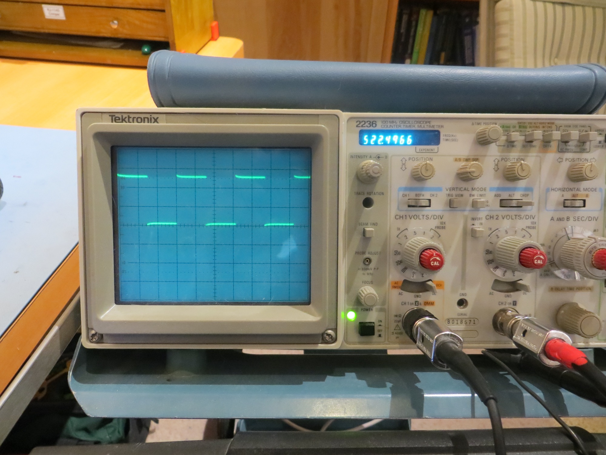
A couple of quick bench-top tests convinced me I was on the right track; At 1m separation between the IR LED/reflector combination and the robot, I was able to drive the robot’s phototransistors into saturation (i.e. an analog input reading of about 20 out of 1024 max), where before I was lucky to get it down to 100 or so.  However, this only happened when I got the LED positioned at the reflector focal point, which was tricky to do by hand, but not too bad for a first try!

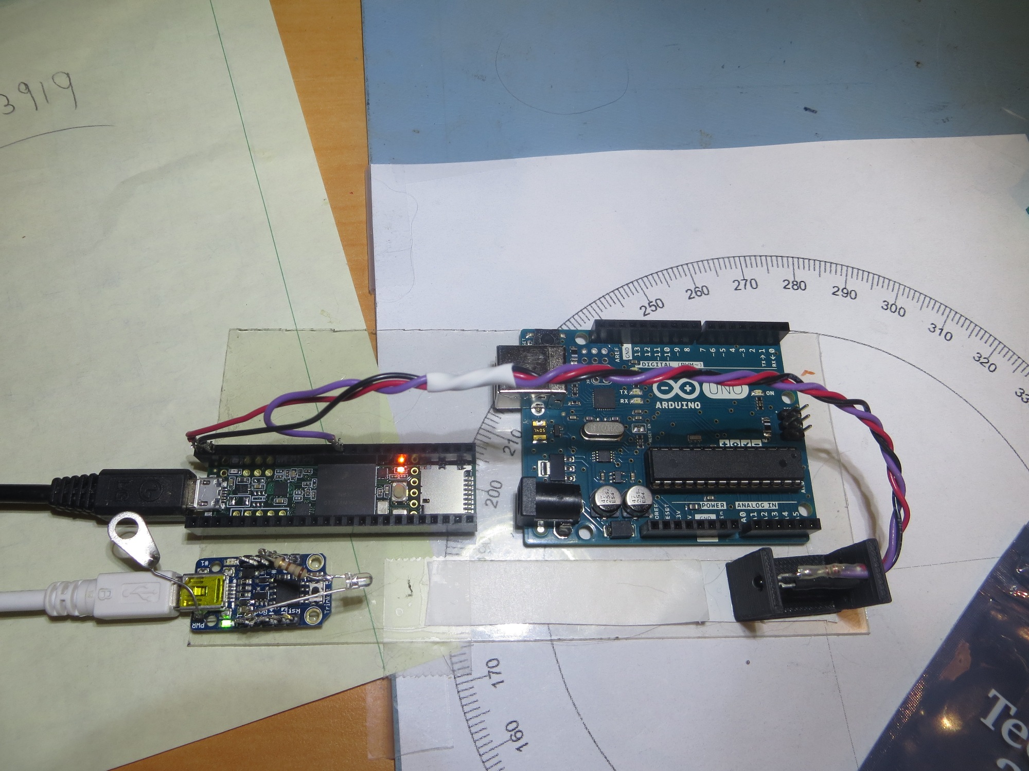
Next, I tried incorporating the reflector idea into the current charging station IR LED/charging probe fixture, as shown in the following photo. This was much closer to what I wanted, but it still was too difficult to get the IR LED positioned correctly, and this was made even more difficult by the fact that I literally could not see what I was doing – it’s IR after all!

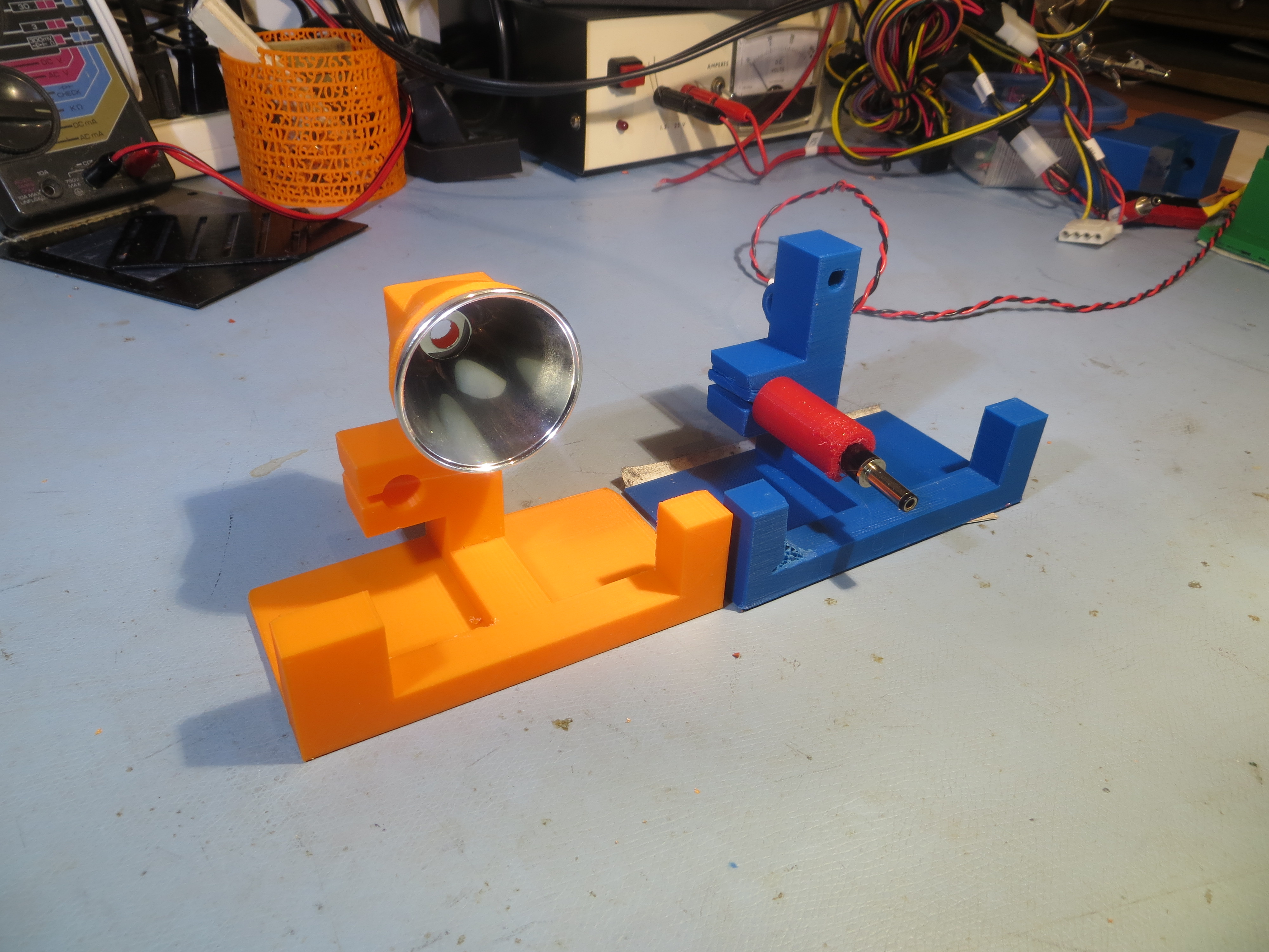
New reflector and old charging station fixture designs

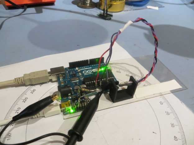
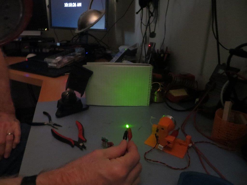
However, the reflector focusing performance should be (mostly) the same for IR and visible wavelengths, so I should be able to use a visible-wavelength LED for initial testing, at least.  So, I set up a small white screen 15-20 cm away from the reflector, and used a regular visible LED to investigate focus point position effects.  As the following photos show, the reflector makes quite a difference in energy density.

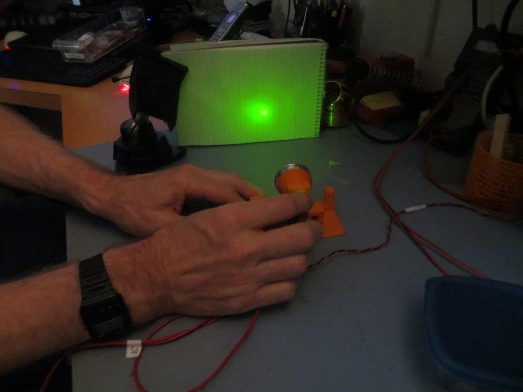
Green visible LED, hand-positioned near the focal point

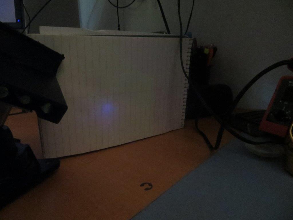
Pattern without the reflector

Next, I used my Canon PowerShot SX260HS digital camera as an IR visualizer so I could see the IR beam pattern. As shown below, the reflector does an excellent job of focusing the available IR energy into a tight beam

IR beam visualized using my Canon PowerShot SX260HS digital camera

IR LED, without reflector

Next, I made another version of the reflector holder, but this time with a way of mounting the LED more firmly at (or as near as I could eyeball) the reflector focal point.

Reflector holder modified for more accurate LED mounting

With this modification, I was able to get pretty good focusing without having to fiddle with the LED location, so I set up some range tests on the floor of my lab.  With LED overhead lighting (not incandescent), I was able to get excellent homing performance all the way out to 2m, as shown in the following photos and plots

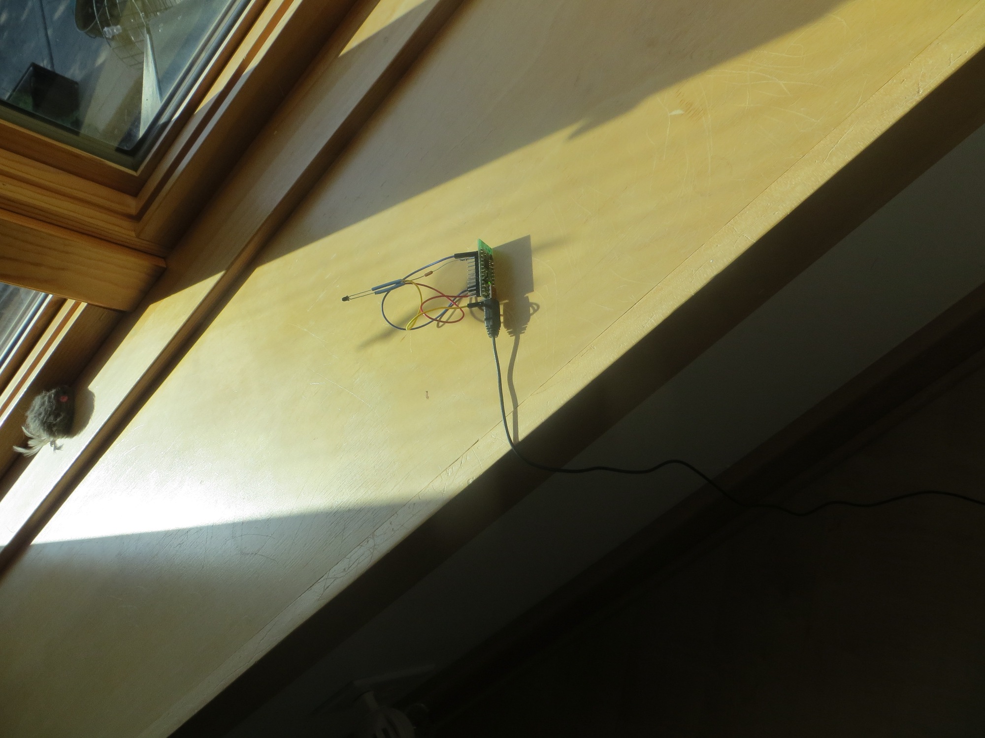
Range testing the IR reflector in the lab. Distance 2m

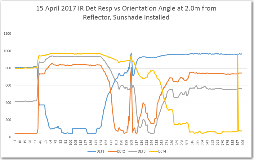
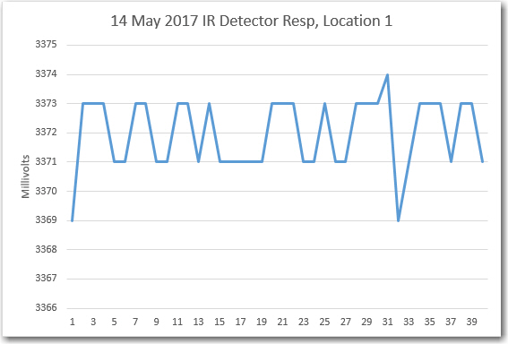
IR Detector response vs orientation at 2m from reflector, in the lab

IR reflector beam pattern at 2m, visualized using digital CCD camera

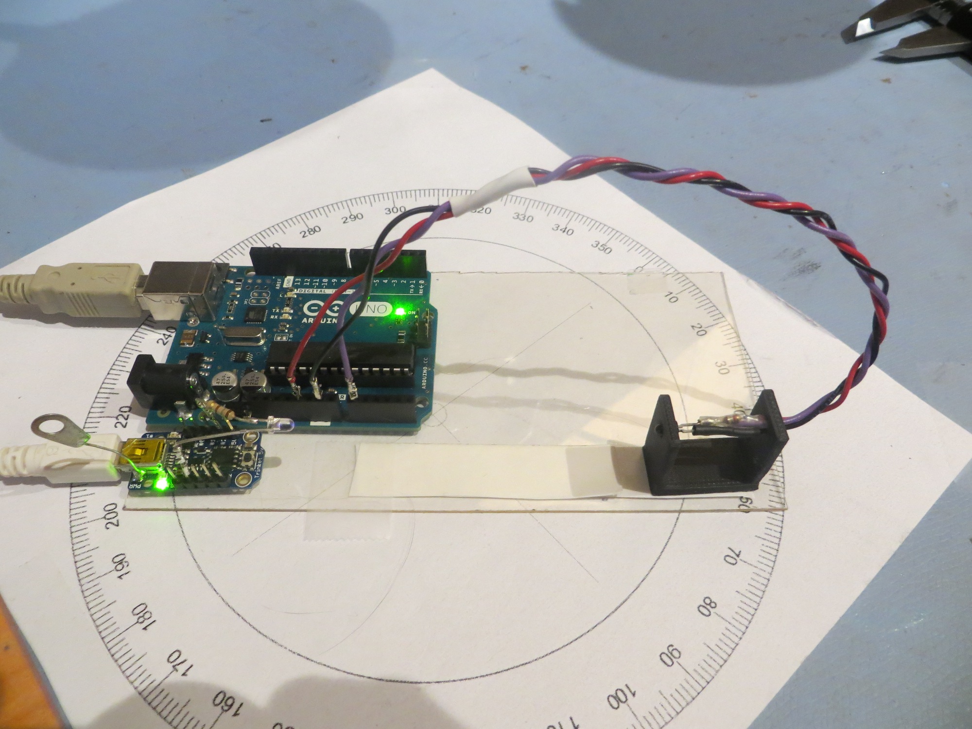
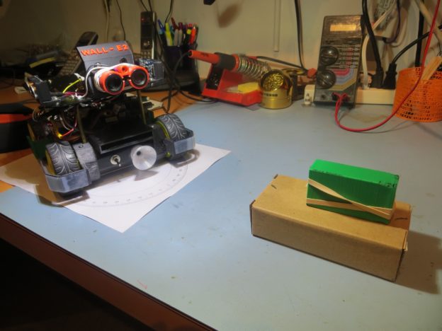
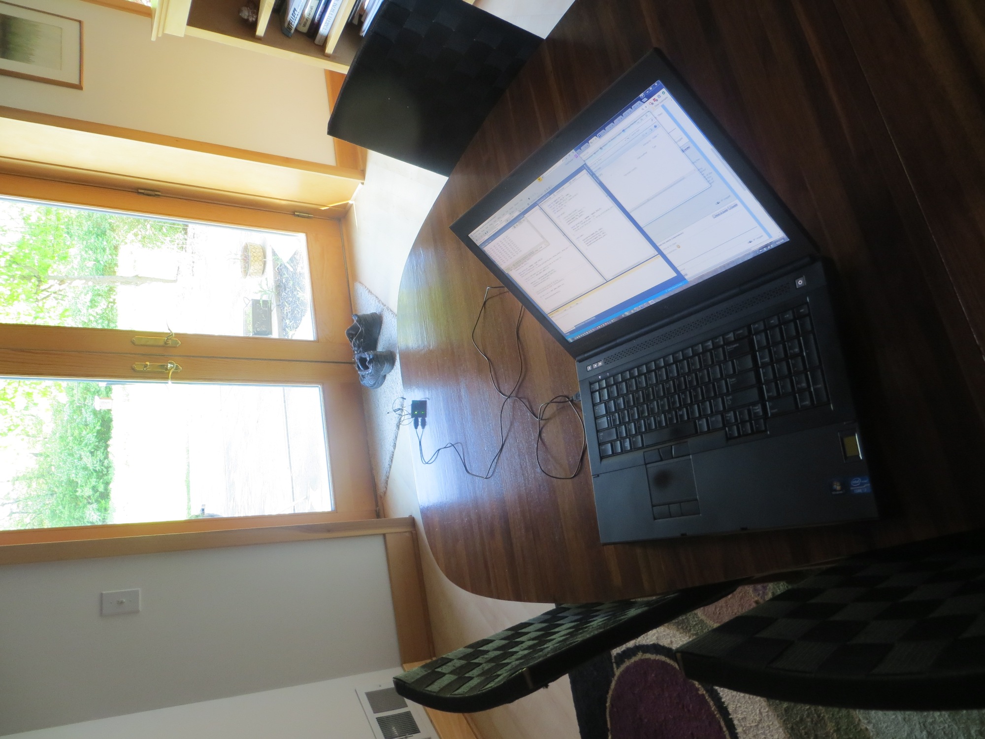
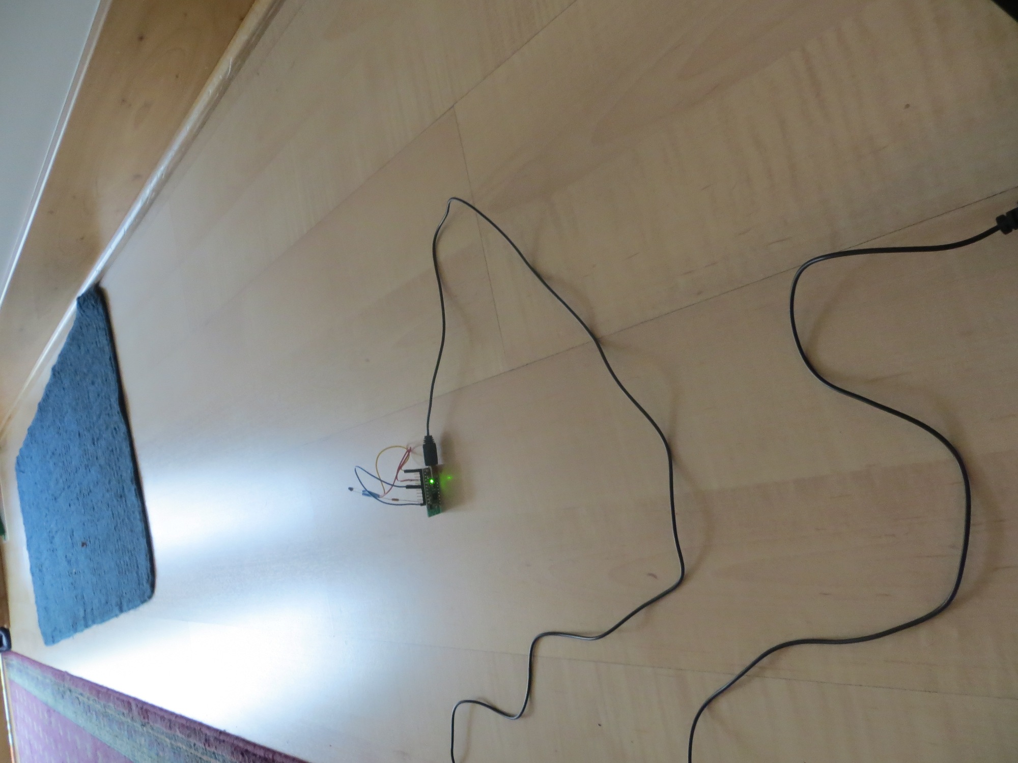
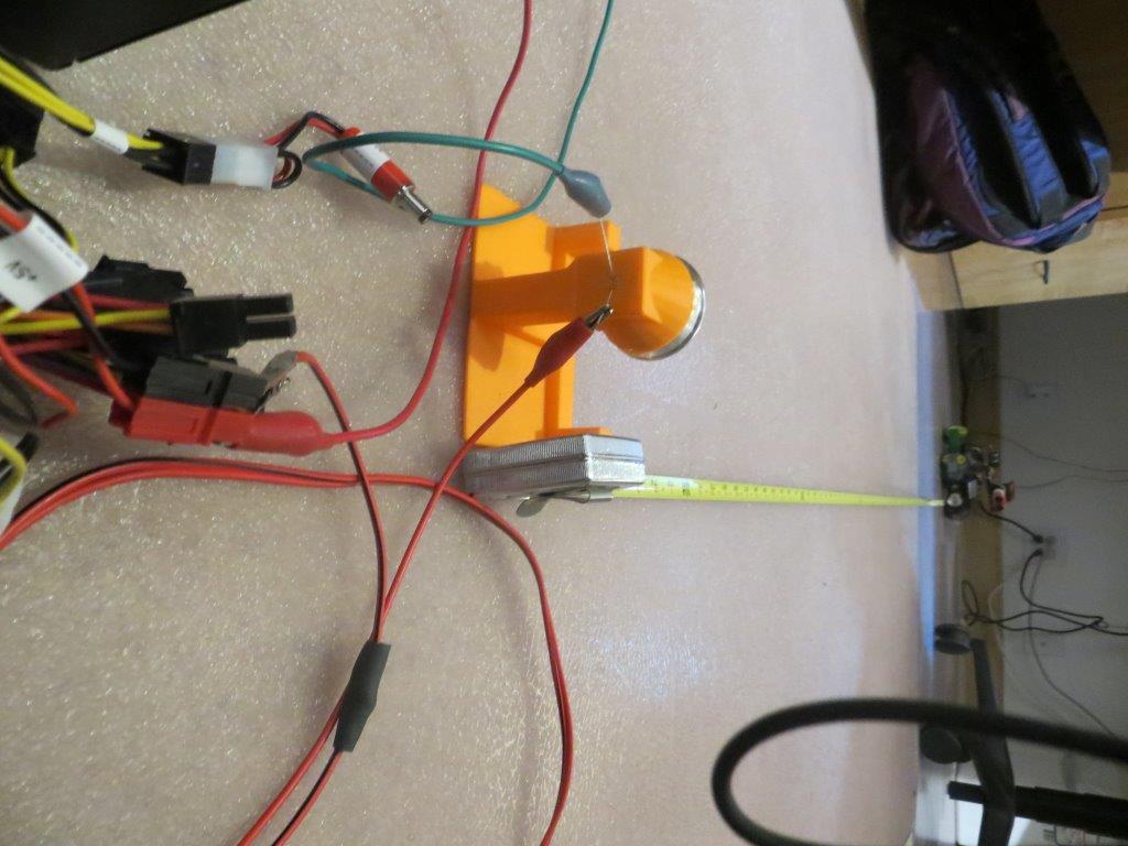
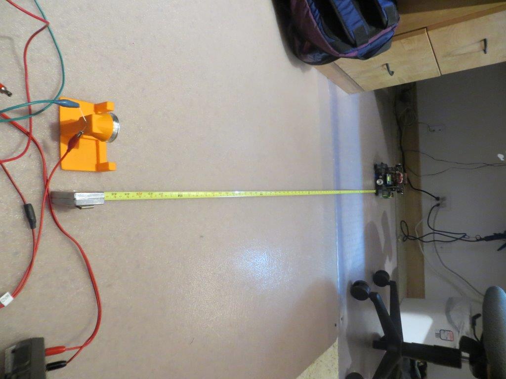
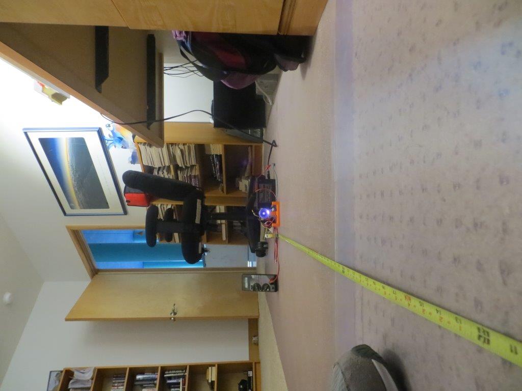
After this, I decided to try my luck again out in our entry hallway, with the dreaded IR interference from the overhead lighting and/or sunlight.   I installed the lead-in rails in the ’tilted’ arrangement, and then performed a response vs orientation test with the robot situated about 2.5m from the IR LED/reflector assembly, in natural daylight illumination with the overhead incandescents OFF.  This produced the curves shown in the plot below.

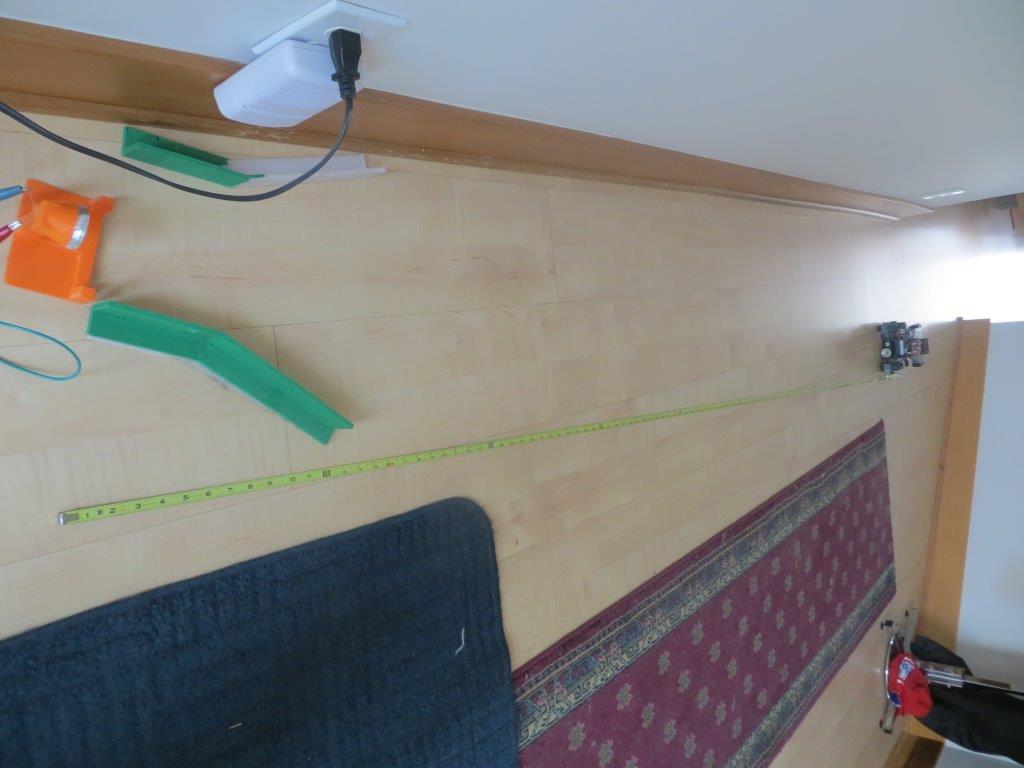
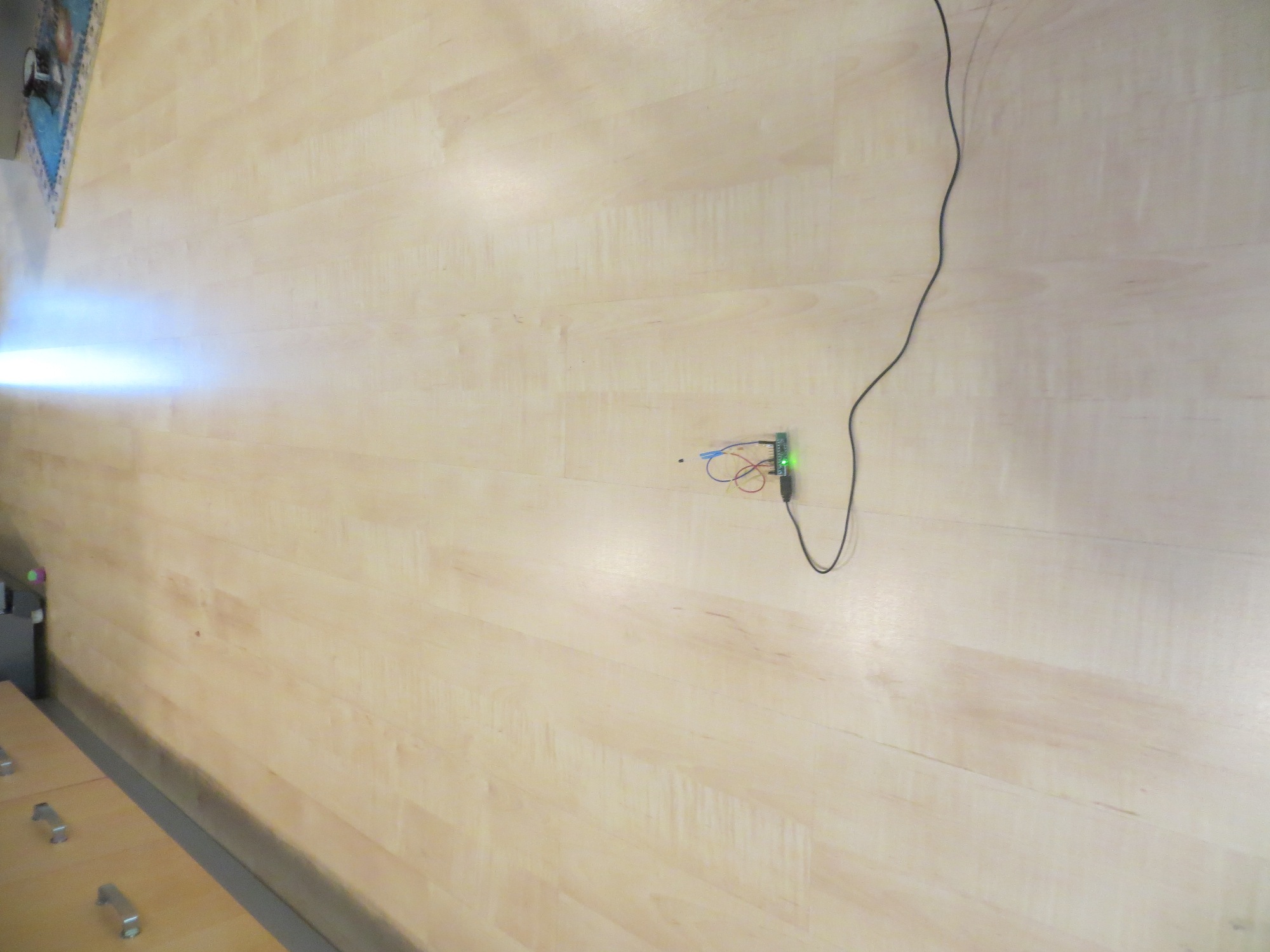
Robot response vs orientation test setup, 2.5 m from tilted lead-in rails & LED/reflector assembly

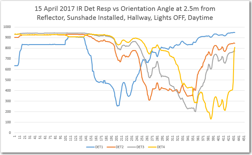
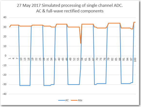
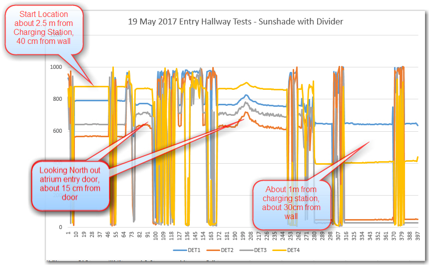
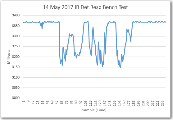
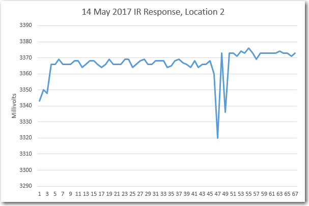
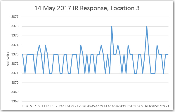
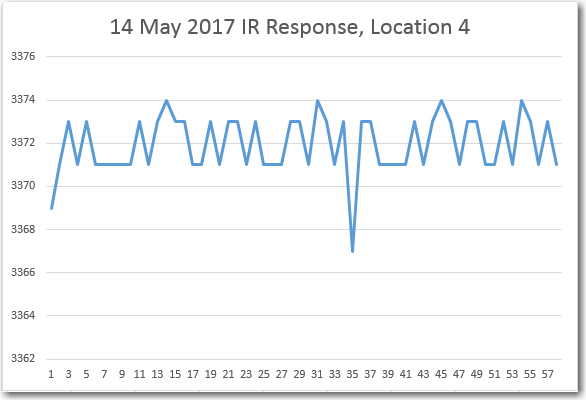
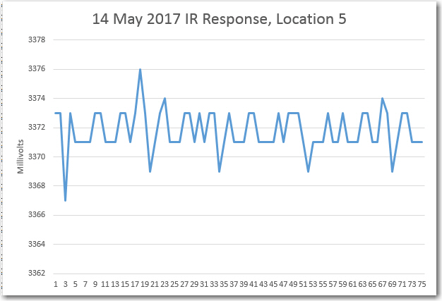
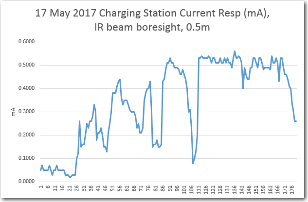
IR detector response vs orientation test, 2.5 m from IR LED/Reflector assembly

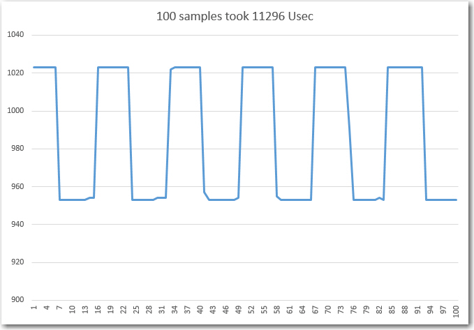
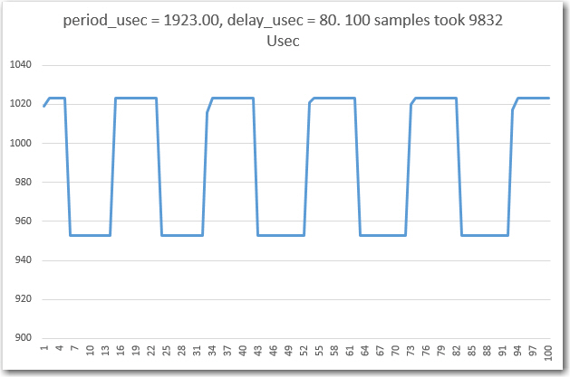
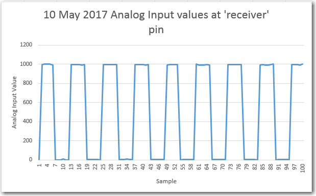
In  the above Excel plot, the individual detector response minimums can be clearly seen, with minimum values in the 200-300 range, and off-axis responses in the 800-1000 range.  This should be more than enough for successful IR homing.

After seeing these positive responses, I ran some homing tests starting from this same general position.  In each run, the robot started off tracking the right-hand wall at about 50 cm  offset.  One run was in daylight with the overhead lights OFF, and another was in daylight with the overhead lights ON.  As can be seen in the videos below.

Both of the above test runs were successful.  The robot started homing on the IR beam almost immediately, and was successfully captured by the lead-in rails.

So, it is clear the reflector idea is a winner – it allows the robot to detect and home in on the IR beam from far enough away to not miss the capture aperture, even in the presence of IR interference from daylight  and/or  overhead incandescent lighting.

Next step – reprint the IR LED reflector holder with the charging probe holder included (I managed to leave it out of the model the last time), and verify that the robot will indeed connect and start charging.