Posted 28 March, 2022
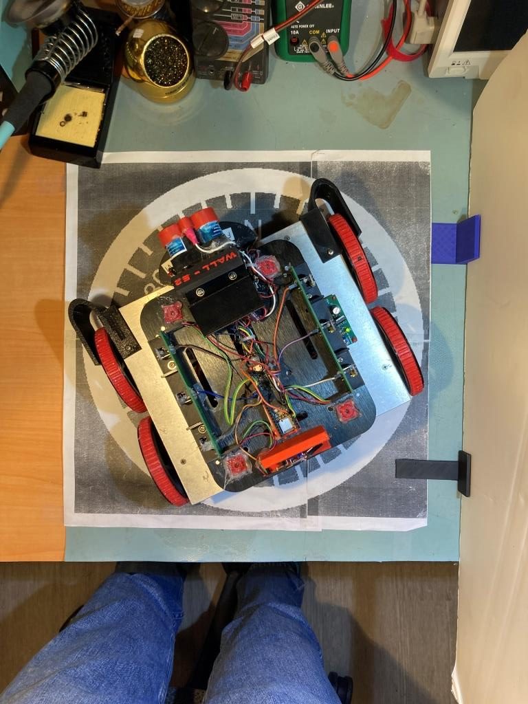
I’ve been working with Wall-E3, my new Teensy 3.5-powered autonomous wall-following robot. I’ve gotten left-wall and right-wall tracking working pretty well, but the transition from one wall to the next (typically right-angle) wall was pretty awkward. The robot basically ran right up to the next wall, stopped, backed up, and then made a right-angle turn to follow the next wall. So, I am trying to make that transition a bit smoother.
After trying a few different ideas, the one I settled on was to use my current very successful ‘SpinTurn()’ function to do the transition. I modified my ‘CheckForAnomalies()’ function to add a check for forward distance less than twice the desired offset distance. When this distance is detected, the robot stops and then makes a right-angle ‘spin’ turn (one sides wheels go forward, the other sides wheels go backward) in the direction away from the currently tracked wall, and then re-enters ‘Track’ mode causing it to track the next wall normally. Here’s a short video showing the process:
Now that I have it working for left-wall tracking, it should be easy to port it to the right-wall tracking condition.
07 April 2022 Update:
Well, as usual, what I thought would be easy has turned out to be anything but. I was able to port the left wall tracking algorithm to the right side, but as I was testing the result, I noticed that Wall-E3 doesn’t really track the right (or left, for that matter) wall. After it ‘captures’ the desired wall offset and turns back to the parallel orientation, it basically goes straight ahead (same speed applied to both side’s motors). If the initial orientation is close to parallel, it looks like it is tracking, but it isn’t.
So, I tried a number of ideas to actually get it to track the desired offset, but they all resulted in poor-to-catastrophic tracking. After working the problem, I began to see that, as always, the issue is the errors associated with the VL53L0X sensor distance measurements. There are two distinct types of errors – an initial ‘calibration’ error associated with sensor-to-sensor variation, and the measurement error that occurs when the robot isn’t oriented parallel to the measured surface.
Calibration Errors:
Each individual VL53L0X sensor gets a slightly different value for the distance to the target, and sometimes ‘slightly’ can be pretty big – 2-3cm at 20cm, for instance. Up until now I had been ignoring these errors, but the time had come to do something about. So, as I always do when troubleshooting an issue, I started taking data. I ran a bunch of trials for all seven VL53L0X sensors at various distances. After gathering the data, I used Excel’s curve-fitting capability to fit a linear equation to the points, as shown below:
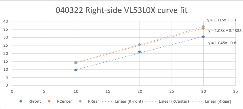
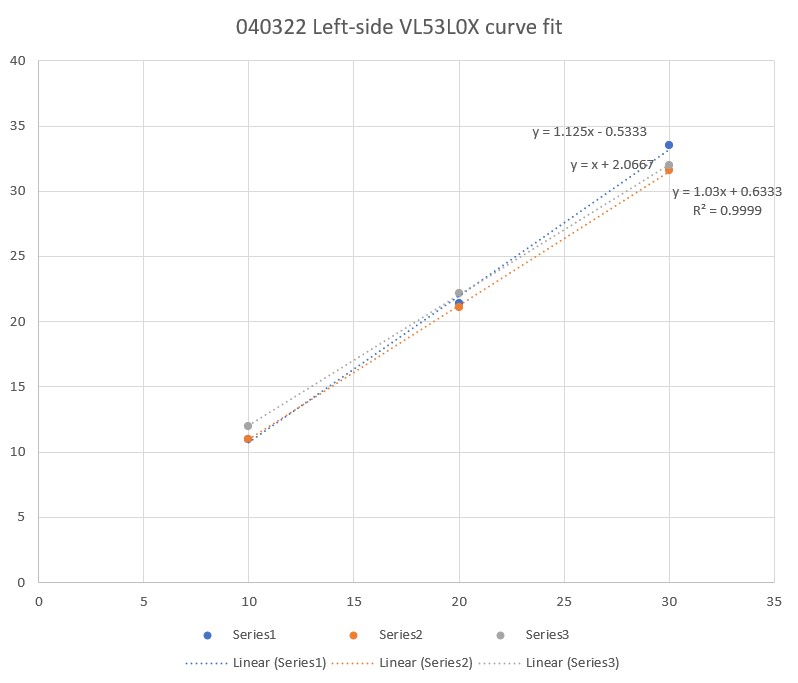
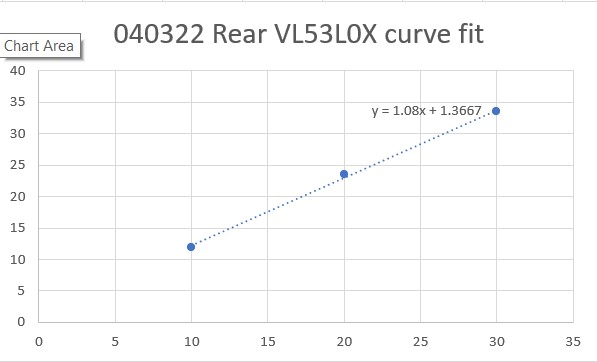
The linear-fit equations gave me a starting point, but they still had to be tweaked a bit to provide the best possible match between what the VL53L0X sensor reported and the actual measurement. Again I used Excel to tweak the equations to give the best match as shown below:
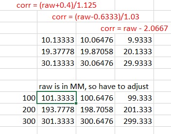
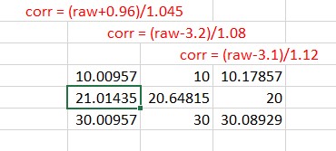
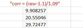
The expressions shown in red are the ones used to correct the VL53L0X-measured distances to be as close as possible to the actual distances (10cm, 20cm, 30cm).
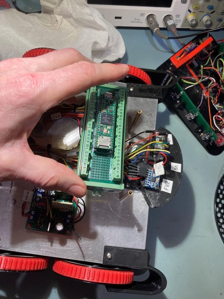
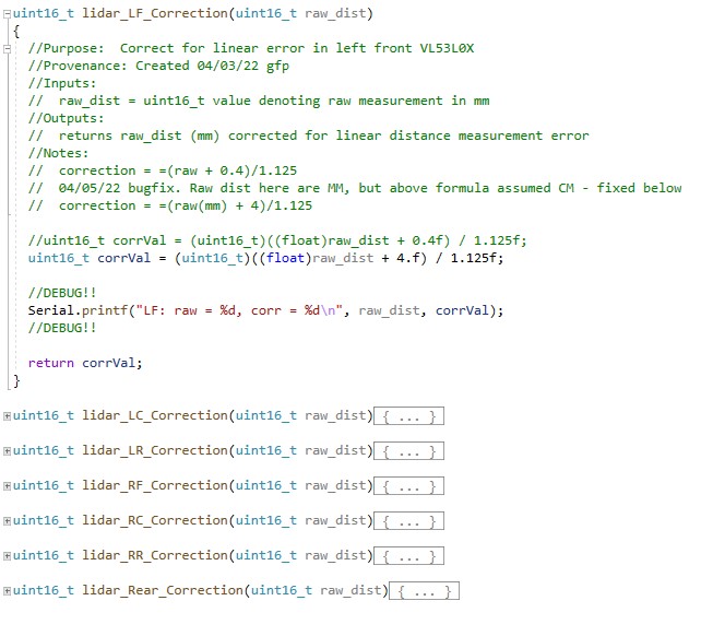
The above corrections were coded into a set of seven ‘correction’ functions for the Teensy 3.5 program that manages the two VL53L0X arrays and the single VL53L0X rear distance sensor.
While this did, indeed, solve a lot of problems – especially with the calculations for wall offset capture initial approach angle, it still didn’t entirely address Wall-E3’s inconsistent offset tracking performance.
Orientation Angle Induced Errors:
Wall-E3 tracks walls by offset by comparing the center VL53L0X measurement to the desired offset, and adjusting the left/right motor speeds to turn the robot in the desired direction. Unfortunately, the turn also throws off the measurements as now the sensors are pointing off-perpendicular, and return a different distance than the actual robot-to-wall perpendicular distance. I tried adjusting the PID controller algorithm to control the robot’s steering angle rather than the offset distance, and then calculating a new steering angle each time – this worked, but not very well.
So, the solution (I think) is to come up with a distance correction factor for off-perpendicular orientations. Going through the trigonometry, I came up with this expression:
I programmed this into the following function:
|
1 2 3 4 5 6 7 8 9 10 |
uint16_t OrientCorr(uint16_t meas_dist, float steerval) { //double corr_ang_rad = atan2(100*steerval,83.f); //83mm between front & rear sensors double corr_ang_rad = atan2(100*steerval,83.f); //83mm between front & rear sensors double corr_dist = meas_dist * cos(corr_ang_rad); myTeePrint.printf("OrientCorr: meas = %d, steer = %2.2f, corr_ang_rad = %2.2f, corr_dist = %2.2f\n", meas_dist, steerval, corr_ang_rad, corr_dist); return (uint16_t)round(corr_dist); } |
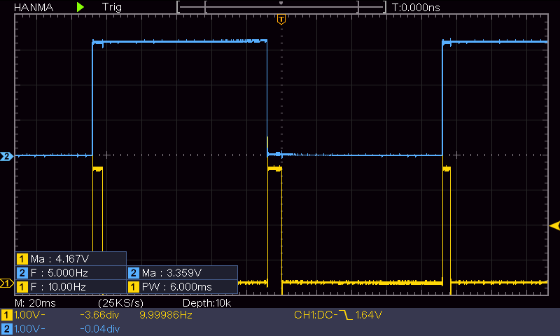
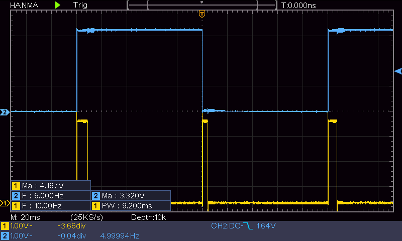
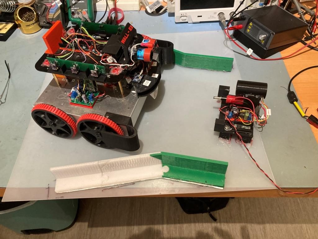
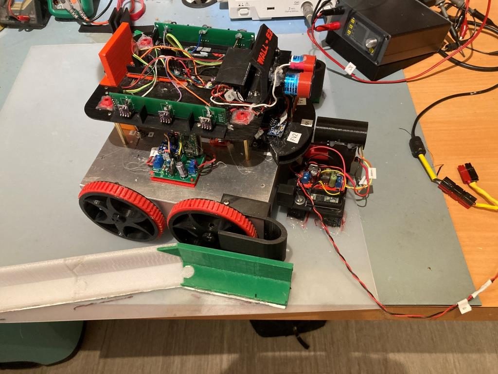
and then ran some tests to verify that the correction algorithm was having the desired effect. Here’s the setup:
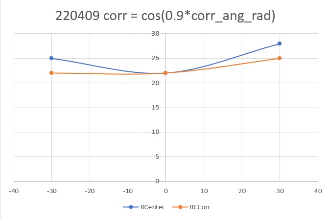
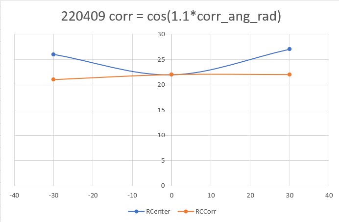
and here are some Excel plots showing the results

As can be seen from the above plot, the corrected distance (gray curve) is pretty constant for angles of -30, 0 and +30 degrees.
09 April 2022 Update:
I have been thinking about the above orientation angle induced errors issue for a couple of days. I wasn’t really happy with that correction as shown in the above Excel plot, and it occurred to me that I didn’t really have to strictly abide by the above correction expression derived from the actual geometry. What I really wanted was a correction that would be accurate at low (or zero) offset angles, but would slightly over-correct for orientation angles in the +/- 30 deg range. In this way, when the PID engine adjusts the motor speeds to correct for an offset error, the system doesn’t try to run away. In fact, for a slight overcorrection algorithm, the center distance reported by the robot might actually go down rather than up for off-perpendicular angles. This would tend to make the PID think that it was over-correcting instead of under-correcting as it does with uncorrected distance reporting.
So, I went back to my test setup, and made some more measurements of corrected vs uncorrected center distances for -30, 0, and 30 degree orientations, for varying values of ‘tweak’ values in he correction expression, as shown in the Excel plots below:
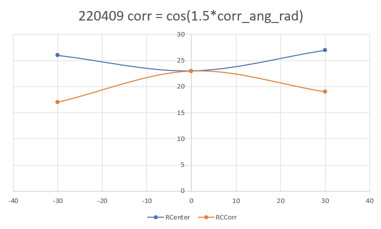
Out of the above correction values, I like the “cos(1.1*corr_ang_rad)” configuration the best. The correction doesn’t modify the center distance at all for the parallel case, and produces a very slight over-correction at the +/- 30 degree orientation cases.
I added the ‘1.1*’ correction to the ‘OrientCorr()’ function and performed another right wall tracking test in my office ‘sandbox’ as shown in the short video below:
Here is the telemetry output for this run:
|
1 2 3 4 5 6 7 8 9 10 11 12 13 14 15 16 17 18 19 20 21 22 23 24 25 26 27 28 29 30 31 32 33 34 35 36 37 38 39 40 41 42 43 44 45 46 47 48 49 50 51 52 53 54 55 56 57 58 59 60 61 62 63 64 65 66 67 68 69 70 71 72 73 74 75 76 77 78 79 80 81 82 83 84 85 86 87 88 89 90 91 92 93 94 95 96 97 98 99 100 101 102 103 104 105 106 107 108 109 110 111 112 113 114 115 116 117 118 119 120 121 122 123 124 125 126 127 128 129 130 131 132 133 134 135 136 137 138 139 140 141 142 143 144 145 146 147 148 149 150 151 152 153 154 155 156 157 158 159 160 161 162 163 164 165 166 167 168 169 170 171 172 173 174 175 176 177 178 179 180 181 182 183 184 185 186 187 188 189 190 191 192 193 194 195 196 197 198 199 200 201 |
In TrackRightWallOffset with Kp/Ki/Kd = 300.00 0.00 10.00 In TrackRightWallOffset with RR/RC/RF = 30 30 30 straight window = 8 cm R/C/F dists = 30 30 30 Steerval = 0.020, WallAngle = 1.14, Inside In SpinTurn(CCW, 28.86, 45.00) R/C/F dists = 27 30 30 Steerval = 0.350, WallOrientDeg = 20.00 approach start: orient angle = 20.000, tgt_distCm = 40 At start - err = prev_err = -10 R/C/F dists = 27 30 30 Steerval = 0.350, OrientDeg = 20.00, err/prev_err = -10 R/C/F dists = 27 30 30 Steerval = 0.350, OrientDeg = 20.00, err/prev_err = -10 Msec RFront RCtr RRear Orient Front Rear Err P_err 68368: Error in GetFrontDistCm() - 0 replaced with 60 68384 31 30 28 17.1 118 46 -10 -10 68496 34 33 30 22.3 125 56 -7 -10 68609 36 36 32 24.0 119 60 -4 -7 68720 39 38 34 28.0 115 66 -2 -4 68831 44 41 36 44.0 108 68 1 -2 At end of offset capture - prev_res*res = -2 correct back to parallel (Right side): RF/RC/RR/Orient = 44 41 36 44.00 In SpinTurn(CW, 44.00, 30.00) TrackRightWallOffset: Start tracking offset of 40.00cm with Kp/Ki/Kd = 300.00 0.00 10.00 Msec LF LC LR RF RC RR F Fvar R Rvar Steer Set Output LSpd RSpd 69557 728 794 816 49 47 50 95 10899 73 39363 -0.10 -0.07 8.70 66 83 69657 728 794 816 50 51 52 99 10901 80 39332 -0.18 -0.11 20.60 54 95 69756 728 794 816 50 48 50 93 10910 86 39318 0.00 -0.08 -22.50 97 52 69858 728 794 816 49 46 48 90 10917 94 39277 0.09 -0.06 -44.30 119 30 69958 728 794 816 46 44 47 86 10927 87 39265 -0.10 -0.04 15.90 59 90 70055 728 114 816 44 45 45 76 10956 102 39252 -0.11 -0.05 18.00 57 93 70157 728 108 816 43 41 43 77 10976 819 48383 -0.02 -0.01 3.50 71 78 70255 728 109 816 39 38 40 74 10994 123 48334 -0.09 0.02 32.00 43 107 70357 109 99 816 36 36 38 70 11023 750 55303 -0.19 0.04 67.80 7 127 70455 112 103 816 34 33 34 65 11056 104 55318 -0.02 0.07 28.40 46 103 70557 728 116 816 29 30 31 55 11101 819 63702 -0.15 0.10 73.40 1 127 70655 728 120 816 27 27 28 48 11170 106 63708 -0.08 0.13 63.40 11 127 70757 728 794 816 24 24 25 43 11246 110 63715 -0.11 0.15 77.50 0 127 70854 728 794 816 22 22 24 37 11329 118 55334 -0.19 0.15 101.20 0 127 In HandleAnomalousConditions with WALL_OFFSET_DIST_AHEAD error code detected WALL_OFFSET_DIST_AHEAD case detected with tracking case Neither In SpinTurn(CCW, 90.00, 45.00) 71682: glLeftCenterCm = 794 glRightCenterCm = 25 glLeftCenterCm > glRightCenterCm --> Calling TrackRightWallOffset() 71686: TrackRightWallOffset(), glRightFrontCm = 26 In TrackRightWallOffset with Kp/Ki/Kd = 300.00 0.00 10.00 In TrackRightWallOffset with RR/RC/RF = 26 25 26 straight window = 8 cm R/C/F dists = 26 25 26 Steerval = -0.060, WallAngle = -3.43, Inside In SpinTurn(CCW, 33.43, 45.00) R/C/F dists = 26 30 32 Steerval = 0.610, WallOrientDeg = 34.86 approach start: orient angle = 34.857, tgt_distCm = 40 At start - err = prev_err = -8 R/C/F dists = 26 30 32 Steerval = 0.610, OrientDeg = 34.86, err/prev_err = -8 R/C/F dists = 27 33 33 Steerval = 0.580, OrientDeg = 33.14, err/prev_err = -8 Msec RFront RCtr RRear Orient Front Rear Err P_err 72138 33 33 27 33.1 219 25 -7 -8 72254 40 38 31 40.0 195 29 -3 -7 72365 44 43 34 43.4 187 32 3 -3 At end of offset capture - prev_res*res = -9 correct back to parallel (Right side): RF/RC/RR/Orient = 44 43 34 43.43 In SpinTurn(CW, 43.43, 30.00) TrackRightWallOffset: Start tracking offset of 40.00cm with Kp/Ki/Kd = 300.00 0.00 10.00 Msec LF LC LR RF RC RR F Fvar R Rvar Steer Set Output LSpd RSpd 73091 110 112 122 40 38 39 151 11228 29 55621 0.09 0.02 -20.30 95 54 73189 728 110 816 39 40 41 153 11220 35 55688 -0.14 0.00 39.90 35 114 73291 728 112 816 40 38 39 150 11210 37 55762 0.18 0.02 -45.00 120 29 73394 728 111 816 40 38 39 146 11195 36 55854 0.06 0.02 -13.20 88 61 73492 114 115 120 38 37 38 141 11171 41 55917 0.07 0.03 -12.00 87 63 73589 728 113 816 38 38 38 134 11147 50 55921 -0.03 0.02 14.10 60 89 73692 728 116 816 36 37 36 129 11102 56 55913 0.05 0.03 -5.30 80 69 73789 112 115 816 36 35 36 124 11068 55 55971 0.00 0.05 14.30 60 89 73890 728 117 816 35 33 34 118 11028 64 56027 0.14 0.07 -19.80 94 55 73991 728 120 816 34 33 34 112 10988 69 56080 0.00 0.07 19.60 55 94 74090 728 120 816 34 33 32 109 10942 67 56165 0.11 0.07 -10.90 85 64 74189 728 122 816 33 32 32 103 10880 72 56246 0.06 0.08 5.40 69 80 74290 728 122 816 32 31 32 100 10825 85 56296 0.03 0.09 17.60 57 92 74393 728 794 816 32 30 31 92 10778 91 56321 0.10 0.10 0.60 74 75 74489 728 120 816 31 30 31 85 10736 86 56382 -0.01 0.10 31.90 43 106 74589 728 794 816 30 30 30 81 10687 92 56196 -0.01 0.10 33.00 42 108 74689 728 119 816 30 29 30 78 10611 104 56033 -0.01 0.11 35.90 39 110 74793 728 123 816 30 28 29 74 10519 107 55890 0.11 0.12 4.10 70 79 74890 728 122 816 30 29 29 71 10414 107 55749 0.12 0.11 -2.80 77 72 74990 728 794 816 31 29 29 67 10296 119 55629 0.20 0.11 -26.20 101 48 75089 728 115 816 31 30 29 63 10341 122 55523 0.15 0.10 -15.40 90 59 75189 728 119 816 31 31 30 59 10388 111 55452 0.09 0.09 -0.50 75 74 75290 728 115 816 32 31 30 52 10501 750 62042 0.20 0.09 -31.90 106 43 75392 728 119 816 33 31 30 47 10633 819 69966 0.30 0.09 -62.00 127 12 75490 728 123 816 32 32 31 40 10775 819 77492 0.12 0.08 -13.70 88 61 In HandleAnomalousConditions with WALL_OFFSET_DIST_AHEAD error code detected WALL_OFFSET_DIST_AHEAD case detected with tracking case Neither In SpinTurn(CCW, 90.00, 45.00) 76435: glLeftCenterCm = 794 glRightCenterCm = 26 glLeftCenterCm > glRightCenterCm --> Calling TrackRightWallOffset() 76440: TrackRightWallOffset(), glRightFrontCm = 27 In TrackRightWallOffset with Kp/Ki/Kd = 300.00 0.00 10.00 In TrackRightWallOffset with RR/RC/RF = 27 25 26 straight window = 8 cm R/C/F dists = 27 25 26 Steerval = 0.010, WallAngle = 0.57, Inside In SpinTurn(CCW, 29.43, 45.00) R/C/F dists = 26 28 31 Steerval = 0.440, WallOrientDeg = 25.14 approach start: orient angle = 25.143, tgt_distCm = 40 At start - err = prev_err = -9 R/C/F dists = 26 28 31 Steerval = 0.440, OrientDeg = 25.14, err/prev_err = -9 R/C/F dists = 26 28 31 Steerval = 0.440, OrientDeg = 25.14, err/prev_err = -9 Msec RFront RCtr RRear Orient Front Rear Err P_err 76821: Error in GetFrontDistCm() - 0 replaced with 71 76832 32 31 26 33.7 159 40 -9 -9 76944 37 35 30 38.3 171 42 -5 -9 77059 41 39 33 42.3 167 46 -1 -5 77171 43 42 36 42.9 165 50 2 -1 At end of offset capture - prev_res*res = -2 correct back to parallel (Right side): RF/RC/RR/Orient = 43 42 36 42.86 In SpinTurn(CW, 42.86, 30.00) TrackRightWallOffset: Start tracking offset of 40.00cm with Kp/Ki/Kd = 300.00 0.00 10.00 Msec LF LC LR RF RC RR F Fvar R Rvar Steer Set Output LSpd RSpd 77927 728 794 816 42 41 41 116 10841 49 56047 0.08 -0.01 -26.10 101 48 78023 728 794 816 43 41 42 116 10846 46 56107 0.10 -0.01 -32.80 107 42 78126 728 794 816 42 41 45 119 10845 53 56159 -0.26 -0.01 71.40 3 127 78224 728 794 816 42 41 44 117 10841 58 56198 -0.21 -0.01 60.50 14 127 78326 728 794 816 39 39 38 109 10841 54 56270 0.11 0.01 -27.00 102 48 78427 728 794 816 38 36 37 101 10844 56 56357 0.08 0.04 -12.60 87 62 78525 728 794 816 37 35 36 96 10850 65 56427 0.12 0.05 -20.70 95 54 78623 728 794 816 36 36 34 91 10852 72 56493 0.21 0.04 -50.00 125 25 78726 728 794 816 35 35 35 87 10848 71 56543 0.01 0.05 9.90 65 84 78828 728 794 816 35 34 36 84 10841 78 56607 -0.13 0.06 55.50 19 127 78927 728 794 816 34 33 34 80 10836 90 47712 -0.07 0.07 42.50 32 117 79025 728 794 816 33 31 33 74 10836 94 47751 0.04 0.09 15.90 59 90 79124 728 794 816 32 31 31 71 10836 85 40235 0.04 0.09 15.00 60 90 79223 728 794 816 32 31 32 66 10839 103 40236 -0.03 0.09 35.30 39 110 79324 728 794 816 30 29 29 61 10845 110 30500 0.11 0.11 1.20 73 76 79424 728 794 816 30 30 29 56 10855 102 30502 0.18 0.10 -23.20 98 51 79523 728 794 816 31 30 29 50 10862 108 30502 0.27 0.10 -50.10 125 24 79625 728 794 816 31 30 29 43 10877 126 30505 0.21 0.10 -33.60 108 41 79725 728 794 816 31 30 29 38 10884 126 30344 0.18 0.10 -24.30 99 50 In HandleAnomalousConditions with WALL_OFFSET_DIST_AHEAD error code detected WALL_OFFSET_DIST_AHEAD case detected with tracking case Neither In SpinTurn(CCW, 90.00, 45.00) 80675: glLeftCenterCm = 794 glRightCenterCm = 24 glLeftCenterCm > glRightCenterCm --> Calling TrackRightWallOffset() 80680: TrackRightWallOffset(), glRightFrontCm = 25 In TrackRightWallOffset with Kp/Ki/Kd = 300.00 0.00 10.00 In TrackRightWallOffset with RR/RC/RF = 25 24 25 straight window = 8 cm R/C/F dists = 25 24 25 Steerval = 0.050, WallAngle = 2.86, Inside In SpinTurn(CCW, 27.14, 45.00) R/C/F dists = 25 26 28 Steerval = 0.300, WallOrientDeg = 17.14 approach start: orient angle = 17.143, tgt_distCm = 40 At start - err = prev_err = -12 R/C/F dists = 25 26 28 Steerval = 0.300, OrientDeg = 17.14, err/prev_err = -12 R/C/F dists = 25 26 28 Steerval = 0.300, OrientDeg = 17.14, err/prev_err = -12 Msec RFront RCtr RRear Orient Front Rear Err P_err 81023: Error in GetFrontDistCm() - 0 replaced with 85 81031: Error in GetFrontDistCm() - 0 replaced with 85 81035 28 27 24 24.0 85 31 -13 -12 81151 32 32 27 31.4 205 40 -8 -13 81265 35 33 29 34.3 201 45 -7 -8 81378 38 36 31 38.3 196 49 -4 -7 81496 42 38 35 32.0 191 50 -2 -4 81611 45 44 38 17.7 189 55 2 -2 At end of offset capture - prev_res*res = -4 correct back to parallel (Right side): RF/RC/RR/Orient = 45 44 38 17.71 In SpinTurn(CW, 17.71, 30.00) TrackRightWallOffset: Start tracking offset of 40.00cm with Kp/Ki/Kd = 300.00 0.00 10.00 Msec LF LC LR RF RC RR F Fvar R Rvar Steer Set Output LSpd RSpd 82121 113 117 126 44 46 42 134 11189 51 30097 0.19 -0.06 -72.50 127 2 82221 109 111 127 46 45 43 129 11171 57 30079 0.25 -0.05 -89.50 127 0 82321 106 110 119 45 44 43 127 11143 58 30075 0.20 -0.04 -72.60 127 2 82419 108 111 115 46 46 47 127 11105 55 30075 -0.07 -0.06 0.50 74 75 82522 728 114 120 50 49 49 128 11055 61 30081 0.02 -0.09 -31.80 106 43 82621 112 116 816 50 47 50 109 11015 71 30077 -0.03 -0.07 -12.70 87 62 82721 728 794 816 48 46 52 104 10975 69 30073 -0.32 -0.06 75.00 0 127 82820 728 794 126 44 44 46 101 10930 73 30072 -0.18 -0.04 43.20 31 118 82919 728 794 816 43 42 43 110 10854 83 30074 0.05 -0.02 -18.90 93 56 83024 728 121 816 38 37 41 264 11010 82 30086 -0.29 0.03 92.10 0 127 83124 728 794 816 35 35 37 263 11116 83 30090 -0.18 0.05 69.90 5 127 83222 728 794 816 32 32 32 163 10944 85 30098 0.01 0.08 22.60 52 97 83319 728 794 816 30 30 32 87 10840 97 30103 -0.14 0.10 70.30 4 127 83421 728 794 128 30 29 30 82 10725 101 30106 -0.01 0.11 37.20 37 112 83520 728 124 816 29 27 27 81 10581 99 30110 0.18 0.13 -13.30 88 61 83621 728 122 816 28 27 28 77 10425 102 30115 -0.04 0.13 48.80 26 123 83720 728 123 816 28 27 26 73 10555 117 30114 0.17 0.13 -9.90 84 65 83819 728 117 816 28 28 28 68 10656 108 30115 0.05 0.12 19.90 55 94 83919 728 120 816 30 29 28 66 10746 750 30115 0.29 0.11 -51.50 126 23 84018 114 123 816 31 29 27 63 10839 819 30115 0.36 0.11 -74.30 127 0 84119 112 120 816 31 30 28 57 10950 819 30115 0.29 0.10 -57.60 127 17 84217 112 118 126 31 30 30 51 11065 750 37818 0.10 0.10 -1.90 76 73 84317 728 794 816 31 30 31 45 11196 750 45125 0.00 0.10 29.00 46 104 84418 728 122 127 31 29 29 39 11339 819 53775 0.18 0.11 -19.30 94 55 |
Looking at the video and the telemetry, the first leg starts with the normal offset capture maneuver, which ends with the robot about 44cm from the wall. Then it makes a pretty distinct correction toward the wall, overshoots the desired offset, and winds up the leg at about 22cm from the wall.
The second leg again starts with a capture maneuver to about 43cm. Then it stabilizes at about 32cm from the wall – nice.
The third leg maneuvers to about 43cm, and then again stabilizes at about 30cm.
The fourth leg was a bit anomalous, as it appeared to way overcorrect after capturing the desired 40cm offset, but I couldn’t find anything in the telemetry to explain it. It’s a mystery!
It’s clear from the above that I no longer need to correct for orientation angle induced errors during the offset maneuver, as these are now handled by my recent ‘global’ correction code. This will probably help with subsequent offset tracking, as the initial offset should be closer to the offset target at the start of the tracking phase. We’ll see…
After a number of trial runs, I finally settled (as much as anything is ‘settled’ in the Wall-E world) on PID = (400,5,40). Here’s a short video showing performance in this configuration:
And, once again, I still have to port this configuration and code back to the left-side wall tracking configuration. Here’s a short video of left-side wall tracking. Interestingly, my ‘random walk’ PID tuning technique resulted in significantly different PID values (300,0,200) vs (400,5,40) than the right side. No clue why.
At this point, I believe I have gone about as far as I can at the moment for wall tracking. WallE3 now can consistently track the walls in my office ‘sandbox’ using either the left-side or the right-side wall for reference. My plan going forward is to ‘archive’ this version (WallE3_WallTrack_V5) by copying it to a new project. The new project will have the goal of integrating charging station homing/connection into the system.
In preparation, I recently modified the charging station lead-in structure to accommodate the wider wheelbase on WallE3, as shown in the following photo:
17 April 2022 Update:
Well, I spoke too soon when I said above that wall-tracking was “settled”. I ran into a couple of significant problems; first, when the robot is already close to the proper offset, it is supposed to just turn to parallel the wall and then go into tracking mode, but on a number of occasions Wall-E3 ran out of control into the next wall. Secondly, wall tracking was anything but smooth, and I couldn’t get it to reliably track the desired offset. So, back to the drawing board (again).
The ‘close enough’ failures were being caused by a flaw in the ‘RotateToParallelOrientation() routine; as the robot approached the parallel orientation, the PID controller also started slowing the rotation speed, to the point where the robot wasn’t rotating anymore – just going straight ahead. If the actual parallel orientation wasn’t reached, the robot just kept going straight ahead forever – oops! The fix for this was to abandon the RotateToParallelOrientation() subroutine entirely, and just use WallOrientDeg() to get the current angular offset from parallel, and SpinTurn() to turn that angular amount back to parallel. RotateToParallelOrientation() is only used in two places (TrackRight/LeftWallOffset()), so the entire function can be removed as well.
The issue with offset tracking continues to bedevil me. When the robot is turned to approach the offset, the measured distances go the wrong way, so the PID tends to ‘wind up’ and drive the robot toward or away from the wall, rather than smoothly approaching the offset. I thought I had the answer to this by ‘tweaking’ the distance corrections due to off-parallel angles, but sadly, this did not help.
So, I removed the off-angle distance correction and went back to just tracking the steering angle – a value proportional to the difference between the front and rear side distance measurements. Now tracking was much more stable, but the robot traveled in a straight line slightly toward the wall. After a few trials, I realized that the robot was doing exactly what I told it to do – drive the front/back measurement error to zero, but unfortunately ‘zero’ did not equate to ‘parallel’. After scratching my head for a while, I realized that rather than using zero as the setpoint, I should use the value that causes the robot to travel parallel to the wall – which turned out to be about 0.25. Using this value I could increase the Kp value back up to 400 or so, and this resulted in very good tracking of whatever offset resulted from the ‘offset approach’ phase of the tracking algorithm. Just this step was a huge improvement in tracking performance, but it wasn’t quite ‘offset tracking’ yet as it didn’t pay any attention to the actual offset – just the difference between the front and back wall offset measurements.
Once I had this working, I was able to re-incorporate my earlier idea of biasing the actual steering value with a term that is proportional to the actual offset, i.e.
WallTrackSteerVal = glRightSteeringVal + (float)(glRightCenterCm – offsetCm) / 50.f;
This, coupled with the empirically determined steering value setpoint of 0.25 resulted in a very stable, very precise tracking performance, as shown in the short video below and the associated telemetry and Excel plots.
|
1 2 3 4 5 6 7 8 9 10 11 12 13 14 15 16 17 18 19 20 21 22 23 24 25 26 27 28 29 30 31 32 33 34 35 36 37 38 39 40 41 42 43 44 45 46 47 48 49 50 51 52 53 54 55 56 57 58 59 60 61 62 63 64 65 66 67 68 69 70 71 72 73 74 75 76 77 78 79 80 81 82 83 84 85 86 87 88 89 90 91 92 93 94 95 96 97 98 99 100 101 102 103 104 105 106 107 108 109 110 111 112 113 114 115 116 117 118 119 120 121 122 123 124 125 126 127 128 129 130 131 132 133 134 135 136 137 138 139 140 141 142 143 144 145 146 147 148 149 150 151 152 153 154 155 156 157 158 159 160 161 162 163 164 165 166 167 168 169 170 171 172 173 174 175 176 177 178 179 180 181 182 183 184 185 186 187 188 189 190 191 |
approach start: orient angle = 16.571, tgt_distCm = 35 At start: meas_dist = 15, corr_dist = 14, err = prev_err = -21 R/C/F dists = 13 15 15 Steerval = 0.290, OrientDeg = 16.57, err/prev_err = -21 Msec RFront RCtr RRear ODeg ORad c_dist Err P_err 11024 16 15 12 16.6 0.3 14 -21 -21 11135 18 17 14 16.6 0.3 16 -19 -21 11249 20 18 16 16.6 0.3 17 -18 -19 11365 22 22 18 16.6 0.3 21 -14 -18 11480 26 24 21 16.6 0.3 23 -12 -14 11591 29 27 23 16.6 0.3 25 -10 -12 11702 31 30 26 16.6 0.3 28 -7 -10 11814 34 32 29 16.6 0.3 30 -5 -7 11927 36 34 31 16.6 0.3 32 -3 -5 12037 41 38 35 16.6 0.3 36 1 -3 At end of offset capture - prev_res*res = -3 correct back to parallel (Right side): RF/RC/RR/Orient = 41 38 35 16.57 In SpinTurn(CW, 16.57, 30.00) TrackRightWallOffset: Start tracking offset of 40cm with Kp/Ki/Kd = 400.00 0.00 0.00 Msec LF LC LR RF RC RR F Fvar R Rvar Steer Set Output LSpd RSpd 12519 728 794 816 41 39 39 90 11753 60 11683 0.21 0.25 16 59 91 12619 728 794 816 41 39 38 90 11797 70 11628 0.31 0.25 -24 99 51 12719 728 794 816 41 40 38 87 11752 69 11576 0.39 0.25 -56 127 19 12817 728 794 816 41 40 38 87 11588 63 11529 0.37 0.25 -48 123 27 12917 728 113 816 42 40 38 80 11311 70 11482 0.40 0.25 -60 127 14 13016 728 794 816 42 40 40 75 10891 78 11436 0.20 0.25 20 55 95 13118 728 794 816 42 41 40 71 10302 84 11392 0.23 0.25 8 67 83 13220 728 794 816 43 40 39 66 9523 79 11350 0.36 0.25 -44 119 30 13321 728 794 816 42 40 39 62 9693 84 11309 0.22 0.25 12 63 87 13416 728 794 816 42 40 39 59 9870 93 11273 0.27 0.25 -8 83 67 13519 728 794 816 40 39 40 57 10068 93 11237 -0.02 0.25 108 0 127 13618 728 794 816 40 39 38 54 10261 91 11202 0.14 0.25 44 31 119 13716 728 794 816 39 38 38 51 10455 107 11177 0.09 0.25 64 11 127 13817 728 794 816 40 37 37 45 10663 112 11156 0.20 0.25 20 54 95 13918 728 794 816 39 38 36 41 10879 109 11132 0.29 0.25 -16 91 58 14017 728 794 816 40 39 36 35 11109 115 11114 0.38 0.25 -52 127 23 In HandleAnomalousConditions with WALL_OFFSET_DIST_AHEAD error code detected WALL_OFFSET_DIST_AHEAD case detected with tracking case Right In SpinTurn(CCW, 90.00, 45.00) IRHomingValTotalAvg = 199 15351: glLeftCenterCm = 794 glRightCenterCm = 24 glLeftCenterCm > glRightCenterCm --> Calling TrackRightWallOffset() 15355: TrackRightWallOffset(), glRightFrontCm = 26 In TrackRightWallOffset with Kp/Ki/Kd = 400.00 0.00 0.00 In TrackRightWallOffset with RR/RC/RF = 24 24 26 straight window = 8 cm R/C/F dists = 24 24 26 Steerval = 0.170, WallAngle = 9.71, Inside In SpinTurn(CCW, 20.29, 45.00) R/C/F dists = 26 31 32 Steerval = 0.590, WallOrientDeg = 33.71 approach start: orient angle = 33.714, tgt_distCm = 35 At start: meas_dist = 31, corr_dist = 26, err = prev_err = -9 R/C/F dists = 26 31 32 Steerval = 0.590, OrientDeg = 33.71, err/prev_err = -9 Msec RFront RCtr RRear ODeg ORad c_dist Err P_err 15712 33 31 27 33.7 0.6 25 -10 -9 15826 37 34 29 33.7 0.6 28 -7 -10 15940 38 37 32 33.7 0.6 30 -5 -7 16053 42 41 36 33.7 0.6 34 -1 -5 16165 46 44 39 33.7 0.6 36 1 -1 At end of offset capture - prev_res*res = -1 correct back to parallel (Right side): RF/RC/RR/Orient = 46 44 39 33.71 In SpinTurn(CW, 33.71, 30.00) TrackRightWallOffset: Start tracking offset of 40cm with Kp/Ki/Kd = 400.00 0.00 0.00 Msec LF LC LR RF RC RR F Fvar R Rvar Steer Set Output LSpd RSpd 16862 112 110 125 43 43 42 108 11196 64 11178 0.25 0.25 0 75 75 16964 728 110 816 45 43 42 108 11162 65 11179 0.27 0.25 -8 82 67 17060 728 111 127 44 42 40 104 11135 61 11186 0.39 0.25 -56 127 19 17161 110 114 124 42 42 41 102 11105 70 11186 0.19 0.25 24 51 99 17263 728 114 126 44 42 41 100 11077 75 11184 0.30 0.25 -20 94 55 17362 728 115 816 43 42 41 97 11038 71 11186 0.23 0.25 8 67 83 17461 728 116 126 43 41 41 95 10989 77 11185 0.24 0.25 4 71 79 17562 728 113 816 44 41 41 90 10938 86 11183 0.36 0.25 -44 119 30 17664 728 109 124 43 41 41 84 10886 91 11180 0.24 0.25 4 71 79 17763 728 118 816 41 41 41 82 10825 90 11179 0.07 0.25 72 3 127 17860 728 794 127 42 39 39 79 10762 90 11178 0.29 0.25 -16 91 59 17961 728 115 816 41 40 39 73 10708 106 11182 0.23 0.25 8 67 83 18059 728 120 816 42 39 39 69 10656 106 11186 0.21 0.25 16 59 91 18161 728 116 816 41 39 39 64 10608 105 11189 0.15 0.25 40 35 115 18262 728 121 816 40 39 36 60 10550 113 11198 0.35 0.25 -40 115 35 18360 728 121 816 40 38 38 58 10482 124 11217 0.17 0.25 32 42 107 18459 728 121 816 40 38 37 53 10405 117 11228 0.22 0.25 12 63 87 18561 728 121 816 40 38 39 49 10600 750 19677 0.07 0.25 72 3 127 18659 728 794 816 40 39 37 43 10806 819 29443 0.24 0.25 4 71 79 18762 728 120 816 40 39 36 36 11021 819 38752 0.37 0.25 -48 122 27 In HandleAnomalousConditions with WALL_OFFSET_DIST_AHEAD error code detected WALL_OFFSET_DIST_AHEAD case detected with tracking case Right In SpinTurn(CCW, 90.00, 45.00) IRHomingValTotalAvg = 273 19919: glLeftCenterCm = 794 glRightCenterCm = 25 glLeftCenterCm > glRightCenterCm --> Calling TrackRightWallOffset() 19923: TrackRightWallOffset(), glRightFrontCm = 28 In TrackRightWallOffset with Kp/Ki/Kd = 400.00 0.00 0.00 In TrackRightWallOffset with RR/RC/RF = 26 25 28 straight window = 8 cm R/C/F dists = 26 25 28 Steerval = 0.180, WallAngle = 10.29, Inside In SpinTurn(CCW, 19.71, 45.00) R/C/F dists = 25 28 30 Steerval = 0.490, WallOrientDeg = 28.00 approach start: orient angle = 28.000, tgt_distCm = 35 At start: meas_dist = 28, corr_dist = 25, err = prev_err = -10 R/C/F dists = 25 28 30 Steerval = 0.520, OrientDeg = 29.71, err/prev_err = -10 Msec RFront RCtr RRear ODeg ORad c_dist Err P_err 20308 30 28 25 29.7 0.5 24 -11 -10 20420 32 30 26 29.7 0.5 26 -9 -11 20533 33 32 29 29.7 0.5 26 -9 -9 20647 36 33 30 29.7 0.5 28 -7 -9 20761 38 36 32 29.7 0.5 31 -4 -7 20876 41 38 36 29.7 0.5 33 -2 -4 20988 42 42 38 29.7 0.5 36 1 -2 At end of offset capture - prev_res*res = -2 correct back to parallel (Right side): RF/RC/RR/Orient = 42 42 38 29.71 In SpinTurn(CW, 29.71, 30.00) TrackRightWallOffset: Start tracking offset of 40cm with Kp/Ki/Kd = 400.00 0.00 0.00 Msec LF LC LR RF RC RR F Fvar R Rvar Steer Set Output LSpd RSpd 21657 728 794 816 45 42 41 97 10859 68 29659 0.40 0.25 -60 127 14 21758 728 794 816 46 42 43 99 10841 69 29645 0.26 0.25 -4 79 71 21856 728 794 816 44 44 45 98 10811 65 29634 0.04 0.25 84 0 127 21956 728 794 816 45 43 44 95 10782 68 29638 0.14 0.25 44 31 119 22055 728 794 816 44 41 42 91 10754 77 29623 0.21 0.25 16 59 91 22154 728 794 816 42 40 40 85 10722 73 29601 0.21 0.25 16 59 91 22258 728 123 816 42 40 41 82 10686 77 29588 0.14 0.25 44 31 119 22356 728 794 816 42 39 39 77 10648 87 29574 0.24 0.25 4 71 79 22459 728 794 816 41 39 40 74 10604 90 29566 0.16 0.25 36 39 111 22555 728 794 816 40 38 38 70 10564 89 29551 0.19 0.25 24 51 99 22656 728 794 816 39 37 37 68 10513 93 29539 0.08 0.25 68 7 127 22758 728 794 816 40 38 37 64 10459 107 29526 0.22 0.25 12 63 87 22855 728 123 816 42 39 37 60 10395 111 29512 0.49 0.25 -96 127 0 22957 728 121 816 43 42 39 56 10314 106 29497 0.43 0.25 -72 127 3 23057 728 794 816 42 42 39 52 10491 112 29495 0.46 0.25 -84 127 0 23156 728 794 816 43 41 40 49 10673 121 29492 0.32 0.25 -28 103 46 23256 728 794 816 44 41 41 43 10870 126 29488 0.34 0.25 -36 111 39 23355 728 794 816 43 41 40 40 11071 750 37177 0.39 0.25 -56 127 18 In HandleAnomalousConditions with WALL_OFFSET_DIST_AHEAD error code detected WALL_OFFSET_DIST_AHEAD case detected with tracking case Right In SpinTurn(CCW, 90.00, 45.00) IRHomingValTotalAvg = 193 24722: glLeftCenterCm = 794 glRightCenterCm = 30 glLeftCenterCm > glRightCenterCm --> Calling TrackRightWallOffset() 24726: TrackRightWallOffset(), glRightFrontCm = 31 In TrackRightWallOffset with Kp/Ki/Kd = 400.00 0.00 0.00 In TrackRightWallOffset with RR/RC/RF = 30 30 31 straight window = 8 cm R/C/F dists = 30 30 31 Steerval = 0.140, WallAngle = 8.00, Inside In SpinTurn(CCW, 22.00, 45.00) R/C/F dists = 27 29 30 Steerval = 0.300, WallOrientDeg = 17.14 approach start: orient angle = 17.143, tgt_distCm = 35 At start: meas_dist = 29, corr_dist = 28, err = prev_err = -7 R/C/F dists = 27 29 30 Steerval = 0.300, OrientDeg = 17.14, err/prev_err = -7 Msec RFront RCtr RRear ODeg ORad c_dist Err P_err 25109 31 29 27 17.1 0.3 27 -8 -7 25220 32 30 29 17.1 0.3 28 -7 -8 25331 33 31 28 17.1 0.3 29 -6 -7 25446 34 31 30 17.1 0.3 29 -6 -6 25559 35 33 31 17.1 0.3 31 -4 -6 25674 35 34 32 17.1 0.3 32 -3 -4 25787 37 35 32 17.1 0.3 33 -2 -3 25899 39 37 33 17.1 0.3 35 0 -2 At end of offset capture - prev_res*res = 0 correct back to parallel (Right side): RF/RC/RR/Orient = 39 37 33 17.14 In SpinTurn(CW, 17.14, 30.00) TrackRightWallOffset: Start tracking offset of 40cm with Kp/Ki/Kd = 400.00 0.00 0.00 Msec LF LC LR RF RC RR F Fvar R Rvar Steer Set Output LSpd RSpd 26414 111 113 816 41 39 39 99 10861 74 37154 0.21 0.25 16 59 91 26512 113 117 123 41 40 38 100 10811 70 37167 0.27 0.25 -8 83 67 26612 109 113 118 42 38 39 96 10759 70 37170 0.29 0.25 -16 91 58 26714 111 115 124 41 39 38 94 10698 80 37163 0.34 0.25 -36 111 39 26811 109 117 119 40 38 37 88 10645 88 37159 0.27 0.25 -8 83 67 26912 111 113 124 39 38 37 84 10588 84 37172 0.24 0.25 4 71 79 27012 113 117 816 40 38 36 80 10527 87 37178 0.23 0.25 8 67 82 27111 728 120 124 38 37 36 77 10460 98 37165 0.12 0.25 52 23 127 27212 110 116 127 37 35 35 75 10384 101 37171 0.09 0.25 64 11 127 27314 728 114 122 36 36 36 72 10304 101 37178 -0.01 0.25 104 0 127 27412 112 117 816 35 34 33 66 10218 106 37177 0.16 0.25 36 39 111 27511 112 112 816 36 34 33 64 10126 116 37174 0.26 0.25 -4 79 71 27610 728 118 127 38 36 34 62 10261 750 44549 0.28 0.25 -12 87 62 27711 728 117 125 38 38 36 60 10406 750 51599 0.24 0.25 4 71 79 27813 728 112 126 40 37 35 57 10556 819 53316 0.38 0.25 -52 127 23 27911 113 116 816 41 38 35 53 10713 819 53316 0.54 0.25 -116 127 0 28012 728 116 128 41 40 37 46 10888 819 53316 0.36 0.25 -44 119 30 28113 113 114 119 42 40 38 41 11075 750 59737 0.40 0.25 -60 127 14 28212 104 108 120 41 39 39 36 11273 750 65748 0.26 0.25 -4 79 71 |
So now I think I finally (I’ve only been working on this for the last three years!) have a wall tracking algorithm that actually makes sense and does what it is supposed to do – track the wall at a constant offset – yay!!
After getting the right side working, I ported everything back to the left side, with some differences; for the left side approach phase, I wound up using a fudge factor of 10cm vice 5cm to get the approach to stop near the desired offset. Also, the base steering value setpoint was -0.35 instead of +0.25, and the input (WallTrackSteerVal) wound up being
WallTrackSteerVal = glLeftSteeringVal + ((float)glLeftCenterCm - (float)offsetCm) / 25.f; With these settings, Wall-E3 seemed pretty comfortable navigating around my office ‘sandbox’, as shown in the following short video:
Stay tuned,
Frank