Yearly Archives: 2022

Move to a Specified Distance, Revisited

MoveToDesiredFrontDistCm ():

bool MoveToDesiredFrontDistCm(uint16_t offsetCm, float Kp, float Ki, float Kd)
{
  //Purpose: Move forward or backward to a specified front offset distance
  // Inputs:
  //	offsetCm - int denoting desired forward distance offset
  //	Kp,Ki,Kd set at top of program (lines 85-87)
  // Outputs:
  //	Robot moves forward or backward to the desired offset, under PID control
  //Notes:
  //	04/25/21 the Kp/Ki/Kd values are much lower than prescribed by Z-N theory
  //		but I like the slower, more deliberate action.
  //  03/06/22 rev for Teensy 3.5 and PIDCalcs().
  //  05/07/22 bugfix: using the same PID values for 'fwd' and 'bkwrd' positioning means 
  //    using a minus sign here for motor speed.

  float lastError = 0;
  float lastInput = 0;
  float lastIval = 0;
  float lastDerror = 0;

  //DEBUG!!
  gl_pSerPort->printf("MoveToDesiredFrontDistCm(%d): Kp/Ki/Kd= %2.2f/%2.2f/%2.2f\n",
    offsetCm, Kp, Ki, Kd);
  //DEBUG!!

  StopBothMotors();

  //05/30/22 re-init front/back dist arrays to avoid spurious 'stuck' detection
  InitFrontDistArray();
  InitRearDistArray();

  gl_pSerPort->printf("MTFD: at start, tgt = %dcm, curr_dist = %d, front/rear var = %2.1f/%2.1f\n",
    offsetCm, GetFrontDistCm(), glFrontvar, glRearvar);

  gl_pSerPort->printf("Msec\tFdist\tTgtD\terr\tIval\tDerr\tOut\tSpeed\tFVar\tRVar\n");

  UpdateAllEnvironmentParameters();
  //AnomalyCode errcode = NO_ANOMALIES;
  AnomalyCode errcode = CheckForAnomalies();

  MsecSinceLastDistUpdate = 0; //01/08/22 not using ISR anymore
  MsecSinceLastFrontDistUpdate = 0; //added 10/02/22 to slow front LIDAR update rate

  //06/12/22 bugfix: can't have GetFrontDistCm() in while() statement - cuz it gets executed too often
  //OffsetDistVal = (double)GetFrontDistCm();
  //while (abs(GetFrontDistCm() - offsetCm) > 1 && errcode == NO_ANOMALIES)

  while (abs(glFrontCm - offsetCm) > 1 && errcode != STUCK_AHEAD && errcode != STUCK_BEHIND)
  {
    CheckForUserInput();

    if (MsecSinceLastDistUpdate >= MSEC_PER_DIST_UPDATE)
    {
      MsecSinceLastDistUpdate -= MSEC_PER_DIST_UPDATE;

      UpdateAllEnvironmentParameters();
      errcode = CheckForAnomalies();

      OffsetDistVal = (double)GetFrontDistCm();

      //gl_pSerPort->printf("MTFD: in loop, tgt = %dcm, curr_dist = %2.1f\n", offsetCm, OffsetDistVal);

      //OffsetDistOutput = PIDCalcs(OffsetDistVal, (float)offsetCm, lastError,
      //  lastInput, lastIval, lastDerror, OffsetDistKp, OffsetDistKi, OffsetDistKd);
      OffsetDistOutput = PIDCalcs((double)glFrontCm, (float)offsetCm, lastError,
        lastInput, lastIval, lastDerror, Kp, Ki, Kd);

      int16_t speed = (int16_t)OffsetDistOutput;
      //gl_pSerPort->printf("MTFD: in loop, speed = %dcm\n", speed);

      //PIDCalcs out can be negative, must handle both signs
      if (speed >= 0)
      {
        speed = (speed > MOTOR_SPEED_QTR) ? MOTOR_SPEED_QTR : speed;
        speed = (speed <= MOTOR_SPEED_OFF) ? MOTOR_SPEED_OFF : speed;
      }
      else //speed < 0
      {
        speed = (speed < -MOTOR_SPEED_QTR) ? -MOTOR_SPEED_QTR : speed;
      }

      gl_pSerPort->printf("%lu\t%d\t%d\t%2.1f\t%2.1f\t%2.1f\t%2.1f\t%d\t%2.1f\t%2.1f\n",
        millis(), glFrontCm, offsetCm, lastError, lastIval, lastDerror, OffsetDistOutput, speed, glFrontvar, glRearvar);

      //  05/07/22 bugfix: using the same PID values for 'fwd' and 'bkwrd' requires the 
      //    use of a minus sign here for motor speed.
      RunBothMotorsBidirectional(-speed, -speed);
    }
  }

  //05/30/22 only worry about 'stuck' conditions
  //if (errcode == STUCK_AHEAD || errcode == STUCK_BEHIND)
  //{
  //  HandleAnomalousConditions(errcode, TRACKING_NONE);
  //  return false;
  //}

  gl_pSerPort->printf("MTFD: Stopped with front dist = %d and errcode = %s\n", GetFrontDistCm(), AnomalyStrArray[errcode]);
  StopBothMotors();
  return true;
}

100

101

bool MoveToDesiredFrontDistCm(uint16_t offsetCm, float Kp, float Ki, float Kd)

{

//Purpose: Move forward or backward to a specified front offset distance

// Inputs:

// offsetCm - int denoting desired forward distance offset

// Kp,Ki,Kd set at top of program (lines 85-87)

// Outputs:

// Robot moves forward or backward to the desired offset, under PID control

//Notes:

// 04/25/21 the Kp/Ki/Kd values are much lower than prescribed by Z-N theory

// but I like the slower, more deliberate action.

// 03/06/22 rev for Teensy 3.5 and PIDCalcs().

// 05/07/22 bugfix: using the same PID values for 'fwd' and 'bkwrd' positioning means

// using a minus sign here for motor speed.

float lastError = 0;

float lastInput = 0;

float lastIval = 0;

float lastDerror = 0;

//DEBUG!!

gl_pSerPort->printf("MoveToDesiredFrontDistCm(%d): Kp/Ki/Kd= %2.2f/%2.2f/%2.2f\n",

offsetCm, Kp, Ki, Kd);

//DEBUG!!

StopBothMotors();

//05/30/22 re-init front/back dist arrays to avoid spurious 'stuck' detection

InitFrontDistArray();

InitRearDistArray();

gl_pSerPort->printf("MTFD: at start, tgt = %dcm, curr_dist = %d, front/rear var = %2.1f/%2.1f\n",

offsetCm, GetFrontDistCm(), glFrontvar, glRearvar);

gl_pSerPort->printf("Msec\tFdist\tTgtD\terr\tIval\tDerr\tOut\tSpeed\tFVar\tRVar\n");

UpdateAllEnvironmentParameters();

//AnomalyCode errcode = NO_ANOMALIES;

AnomalyCode errcode = CheckForAnomalies();

MsecSinceLastDistUpdate = 0; //01/08/22 not using ISR anymore

MsecSinceLastFrontDistUpdate = 0; //added 10/02/22 to slow front LIDAR update rate

//06/12/22 bugfix: can't have GetFrontDistCm() in while() statement - cuz it gets executed too often

//OffsetDistVal = (double)GetFrontDistCm();

//while (abs(GetFrontDistCm() - offsetCm) > 1 && errcode == NO_ANOMALIES)

while (abs(glFrontCm - offsetCm) > 1 && errcode != STUCK_AHEAD && errcode != STUCK_BEHIND)

{

CheckForUserInput();

if (MsecSinceLastDistUpdate >= MSEC_PER_DIST_UPDATE)

{

MsecSinceLastDistUpdate -= MSEC_PER_DIST_UPDATE;

UpdateAllEnvironmentParameters();

errcode = CheckForAnomalies();

OffsetDistVal = (double)GetFrontDistCm();

//gl_pSerPort->printf("MTFD: in loop, tgt = %dcm, curr_dist = %2.1f\n", offsetCm, OffsetDistVal);

//OffsetDistOutput = PIDCalcs(OffsetDistVal, (float)offsetCm, lastError,

// lastInput, lastIval, lastDerror, OffsetDistKp, OffsetDistKi, OffsetDistKd);

OffsetDistOutput = PIDCalcs((double)glFrontCm, (float)offsetCm, lastError,

lastInput, lastIval, lastDerror, Kp, Ki, Kd);

int16_t speed = (int16_t)OffsetDistOutput;

//gl_pSerPort->printf("MTFD: in loop, speed = %dcm\n", speed);

//PIDCalcs out can be negative, must handle both signs

if (speed >= 0)

{

speed = (speed > MOTOR_SPEED_QTR) ? MOTOR_SPEED_QTR : speed;

speed = (speed <= MOTOR_SPEED_OFF) ? MOTOR_SPEED_OFF : speed;

}

else //speed < 0

{

speed = (speed < -MOTOR_SPEED_QTR) ? -MOTOR_SPEED_QTR : speed;

}

gl_pSerPort->printf("%lu\t%d\t%d\t%2.1f\t%2.1f\t%2.1f\t%2.1f\t%d\t%2.1f\t%2.1f\n",

millis(), glFrontCm, offsetCm, lastError, lastIval, lastDerror, OffsetDistOutput, speed, glFrontvar, glRearvar);

// 05/07/22 bugfix: using the same PID values for 'fwd' and 'bkwrd' requires the

// use of a minus sign here for motor speed.

RunBothMotorsBidirectional(-speed, -speed);

}

//05/30/22 only worry about 'stuck' conditions

//if (errcode == STUCK_AHEAD || errcode == STUCK_BEHIND)

//{

// HandleAnomalousConditions(errcode, TRACKING_NONE);

// return false;

//}

gl_pSerPort->printf("MTFD: Stopped with front dist = %d and errcode = %s\n", GetFrontDistCm(), AnomalyStrArray[errcode]);

StopBothMotors();

return true;

}

Here’s some output from a typical run:

Starting Front/BackSide Motion Test - enter Direction (1 = F, 2 = B, 3 = L, 4 = R), offset, Kp,Ki,Kd
At top of parameter retrieval section
DirStr = 1
OffStr = 60
Moving Front to 60 cm, with PID = (1.50,0.10,0.20)
Enter any key to start

Before MTDFD, FVar = 13062.84
MoveToDesiredFrontDistCm(60): Kp/Ki/Kd= 1.50/0.10/0.20
MTFD: at start, tgt = 60cm, curr_dist = 21, front/rear var = 13328.0/833.0
Msec	Fdist	TgtD	err	Ival	Derr	Out	Speed	FVar	RVar
163417	20	60	40.0	4.0	40.0	56.0	56	13305.6	21444.6
163480	20	60	40.0	8.0	0.0	68.0	68	13974.0	30074.4
163530	20	60	40.0	12.0	0.0	72.0	72	14987.5	40126.6
163581	21	60	39.0	15.9	-1.0	74.6	74	16226.3	49659.8
163628	24	60	36.0	19.5	-3.0	74.1	74	18030.5	58677.5
163680	26	60	34.0	22.9	-2.0	74.3	74	19318.8	67183.6
163729	28	60	32.0	26.1	-2.0	74.5	74	20393.4	73500.8
163779	29	60	31.0	29.2	-1.0	75.9	75	21153.6	79398.7
163830	30	60	30.0	32.2	-1.0	77.4	75	21426.0	84880.5
163878	32	60	28.0	35.0	-2.0	77.4	75	20739.2	89949.6
163929	33	60	27.0	37.7	-1.0	78.4	75	19204.9	94609.4
163980	34	60	26.0	40.3	-1.0	79.5	75	16580.3	98863.2
164032	37	60	23.0	42.6	-3.0	77.7	75	12651.8	104153.8
164081	39	60	21.0	44.7	-2.0	76.6	75	7213.3	107565.6
164130	44	60	16.0	46.3	-5.0	71.3	71	53.6	110581.6
164181	49	60	11.0	47.4	-5.0	64.9	64	67.6	114521.3
164220	53	60	7.0	48.1	-4.0	59.4	59	86.6	117988.8
164281	53	60	7.0	48.8	0.0	59.3	59	99.7	120987.7
164333	57	60	3.0	49.1	-4.0	54.4	54	113.1	123521.6
164382	59	60	1.0	49.2	-2.0	51.1	51	124.7	124450.2
MTFD: Stopped with front dist = 59 and errcode = NO_ANOMALIES
Front	Rear	Left	Right
59	819.10	32.00	779.80
63	819.10	33.00	779.80
65	819.10	34.00	779.80
66	819.10	33.00	779.80
69	750.40	32.00	779.80
67	750.40	32.00	779.80
68	750.40	33.00	779.70
67	819.10	32.00	779.70
68	819.10	32.00	779.80
67	819.10	33.00	779.80

Starting Front/BackSide Motion Test - enter Direction (1 = F, 2 = B, 3 = L, 4 = R), offset, Kp,Ki,Kd

At top of parameter retrieval section

DirStr = 1

OffStr = 60

Moving Front to 60 cm, with PID = (1.50,0.10,0.20)

Enter any key to start

Before MTDFD, FVar = 13062.84

MoveToDesiredFrontDistCm(60): Kp/Ki/Kd= 1.50/0.10/0.20

MTFD: at start, tgt = 60cm, curr_dist = 21, front/rear var = 13328.0/833.0

Msec Fdist TgtD err Ival Derr Out Speed FVar RVar

163417 20 60 40.0 4.0 40.0 56.0 56 13305.6 21444.6

163480 20 60 40.0 8.0 0.0 68.0 68 13974.0 30074.4

163530 20 60 40.0 12.0 0.0 72.0 72 14987.5 40126.6

163581 21 60 39.0 15.9 -1.0 74.6 74 16226.3 49659.8

163628 24 60 36.0 19.5 -3.0 74.1 74 18030.5 58677.5

163680 26 60 34.0 22.9 -2.0 74.3 74 19318.8 67183.6

163729 28 60 32.0 26.1 -2.0 74.5 74 20393.4 73500.8

163779 29 60 31.0 29.2 -1.0 75.9 75 21153.6 79398.7

163830 30 60 30.0 32.2 -1.0 77.4 75 21426.0 84880.5

163878 32 60 28.0 35.0 -2.0 77.4 75 20739.2 89949.6

163929 33 60 27.0 37.7 -1.0 78.4 75 19204.9 94609.4

163980 34 60 26.0 40.3 -1.0 79.5 75 16580.3 98863.2

164032 37 60 23.0 42.6 -3.0 77.7 75 12651.8 104153.8

164081 39 60 21.0 44.7 -2.0 76.6 75 7213.3 107565.6

164130 44 60 16.0 46.3 -5.0 71.3 71 53.6 110581.6

164181 49 60 11.0 47.4 -5.0 64.9 64 67.6 114521.3

164220 53 60 7.0 48.1 -4.0 59.4 59 86.6 117988.8

164281 53 60 7.0 48.8 0.0 59.3 59 99.7 120987.7

164333 57 60 3.0 49.1 -4.0 54.4 54 113.1 123521.6

164382 59 60 1.0 49.2 -2.0 51.1 51 124.7 124450.2

MTFD: Stopped with front dist = 59 and errcode = NO_ANOMALIES

Front Rear Left Right

59 819.10 32.00 779.80

63 819.10 33.00 779.80

65 819.10 34.00 779.80

66 819.10 33.00 779.80

69 750.40 32.00 779.80

67 750.40 32.00 779.80

68 750.40 33.00 779.70

67 819.10 32.00 779.70

68 819.10 32.00 779.80

67 819.10 33.00 779.80

The movement goes OK, and the robot telemetry says it stopped very close to the desired 60cm distance. However, when I measured the actual distance from the ‘wall’ to the robot, I got more like 67 or 68cm, probably indicating that the robot coasted some after the motors were turned off. When I instrumented the code to show the next 10 distance measurements after the exit from the subroutine, it became easy to see that this was the case – the robot coasted from 59 to 67cm. The robot should correct this by going back the opposite way, but it doesn’t because the last measurement (59cm) fits inside the 59-61cm ‘basket’ for subroutine termination (the ‘while’ loop termination criteria).

So, I thought what I could do is check the reported front distance after function exit, and just call it again if the robot had coasted too far from the target. The second run should get much closer, as the starting error term would be much smaller. So now the test code looks like this:

        gl_pSerPort->printf("Before MTDFD, FVar = %2.2f\n", glFrontvar);

        MoveToDesiredFrontDistCm(Offset,Kp,Ki,Kd);

        //show 10 distances after stop
        gl_pSerPort->printf("Front\tRear\tLeft\tRight\n");
        for (size_t i = 0; i < 10; i++)
        {
          GetRequestedVL53l0xValues(VL53L0X_ALL);
          glFrontCm = GetFrontDistCm();
          gl_pSerPort->printf("%d\t%2.2f\t%2.2f\t%2.2f\n",
            glFrontCm, glRearCm, glLeftCenterCm, glRightCenterCm);
          delay(100);
        }

        if (abs(glFrontCm - Offset) > 1)
        {
          gl_pSerPort->printf("Second time through MTDFD with error = %d\n", abs(glFrontCm - Offset));
          MoveToDesiredFrontDistCm(Offset,Kp/2,Ki,Kd);
        }

gl_pSerPort->printf("Before MTDFD, FVar = %2.2f\n", glFrontvar);

MoveToDesiredFrontDistCm(Offset,Kp,Ki,Kd);

//show 10 distances after stop

gl_pSerPort->printf("Front\tRear\tLeft\tRight\n");

for (size_t i = 0; i < 10; i++)

{

GetRequestedVL53l0xValues(VL53L0X_ALL);

glFrontCm = GetFrontDistCm();

gl_pSerPort->printf("%d\t%2.2f\t%2.2f\t%2.2f\n",

glFrontCm, glRearCm, glLeftCenterCm, glRightCenterCm);

delay(100);

}

if (abs(glFrontCm - Offset) > 1)

{

gl_pSerPort->printf("Second time through MTDFD with error = %d\n", abs(glFrontCm - Offset));

MoveToDesiredFrontDistCm(Offset,Kp/2,Ki,Kd);

}

This should have worked well, except when I tried it, the function exited with a ‘STUCK_AHEAD’ error – oops! Here’s a run going from 60 from 30cm:

Moving Front to 30 cm, with PID = (1.50,0.10,0.20)
Enter any key to start
Got 51
Got 46
Got 46
Got 46
Got 255
Before MTDFD, FVar = 12228.16
MoveToDesiredFrontDistCm(30): Kp/Ki/Kd= 1.50/0.10/0.20
MTFD: at start, tgt = 30cm, curr_dist = 65, front/rear var = 13328.0/833.0
Msec	Fdist	TgtD	err	Ival	Derr	Out	Speed	FVar	RVar
4812697	64	30	-34.0	-3.4	-34.0	-47.6	-47	11618.7	23386.2
4812746	66	30	-36.0	-7.0	-2.0	-60.6	-60	11452.8	23271.3
4812800	65	30	-35.0	-10.5	1.0	-63.2	-63	11682.5	33698.9
4812849	64	30	-34.0	-13.9	1.0	-65.1	-65	12236.1	41759.9
4812899	63	30	-33.0	-17.2	1.0	-66.9	-66	13316.3	49390.2
4812944	60	30	-30.0	-20.2	3.0	-65.8	-65	14265.6	56593.1
4812981	61	30	-31.0	-23.3	-1.0	-69.6	-69	15163.5	63372.0
4813049	60	30	-30.0	-26.3	1.0	-71.5	-71	15891.4	69730.2
4813095	57	30	-27.0	-29.0	3.0	-70.1	-70	16326.1	77314.4
4813148	55	30	-25.0	-31.5	2.0	-69.4	-69	16138.6	84400.2
4813199	55	30	-25.0	-34.0	0.0	-71.5	-71	15176.2	90991.4
4813235	52	30	-22.0	-36.2	3.0	-69.8	-69	13311.0	97091.6
4813297	50	30	-20.0	-38.2	2.0	-68.6	-68	10317.8	101237.0
4813346	49	30	-19.0	-40.1	1.0	-68.8	-68	5972.6	104982.1
4813396	44	30	-14.0	-41.5	5.0	-63.5	-63	40.8	108330.4
MTFD: Stopped with front dist = 44 and errcode = STUCK_AHEAD

Moving Front to 30 cm, with PID = (1.50,0.10,0.20)

Enter any key to start

Got 51

Got 46

Got 255

Before MTDFD, FVar = 12228.16

MoveToDesiredFrontDistCm(30): Kp/Ki/Kd= 1.50/0.10/0.20

MTFD: at start, tgt = 30cm, curr_dist = 65, front/rear var = 13328.0/833.0

Msec Fdist TgtD err Ival Derr Out Speed FVar RVar

4812697 64 30 -34.0 -3.4 -34.0 -47.6 -47 11618.7 23386.2

4812746 66 30 -36.0 -7.0 -2.0 -60.6 -60 11452.8 23271.3

4812800 65 30 -35.0 -10.5 1.0 -63.2 -63 11682.5 33698.9

4812849 64 30 -34.0 -13.9 1.0 -65.1 -65 12236.1 41759.9

4812899 63 30 -33.0 -17.2 1.0 -66.9 -66 13316.3 49390.2

4812944 60 30 -30.0 -20.2 3.0 -65.8 -65 14265.6 56593.1

4812981 61 30 -31.0 -23.3 -1.0 -69.6 -69 15163.5 63372.0

4813049 60 30 -30.0 -26.3 1.0 -71.5 -71 15891.4 69730.2

4813095 57 30 -27.0 -29.0 3.0 -70.1 -70 16326.1 77314.4

4813148 55 30 -25.0 -31.5 2.0 -69.4 -69 16138.6 84400.2

4813199 55 30 -25.0 -34.0 0.0 -71.5 -71 15176.2 90991.4

4813235 52 30 -22.0 -36.2 3.0 -69.8 -69 13311.0 97091.6

4813297 50 30 -20.0 -38.2 2.0 -68.6 -68 10317.8 101237.0

4813346 49 30 -19.0 -40.1 1.0 -68.8 -68 5972.6 104982.1

4813396 44 30 -14.0 -41.5 5.0 -63.5 -63 40.8 108330.4

MTFD: Stopped with front dist = 44 and errcode = STUCK_AHEAD

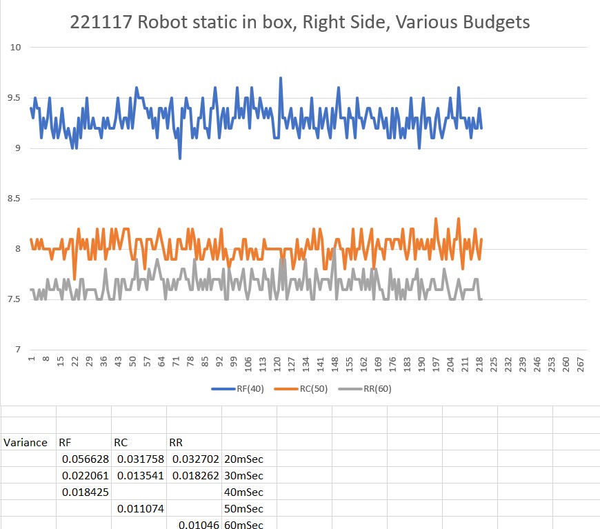
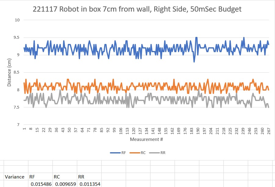
The ‘stuck’ checks have to be there because the robot can’t ‘see’ obstacles that are too low to interrupt the front LIDAR beam, or aren’t directly in the line of sight, but how to manage? The ‘stuck’ checks depend on a variance calculation on the last 50 measurements (held in a bit-bucket array), so I began to wonder why the front variance was decreasing so rapidly while the rear variance wasn’t (one would think they would behave more or less the same). So I went back and printed out the front & back distance array contents after each run, and saw that the reason the front variance was decreasing so rapidly was because I was using a 50mSec time interval, meaning the 50-element array was getting filled in 2500mSec – or about 2.5sec. So, in order to get more variance in a normal run, either the run has to be done at a faster speed (leading to more overshoot) or the timing interval has to be increased. In earlier work I had discovered that the front LIDAR system produces errors for long distance measurements when using short measurement intervals, so I increased the measurement interval from 50 to 200mSec, and now the variance decreases at a much slower rate – yay!

With the longer 200mSec measurement interval, the movement routine now has time to adjust for overshoots, as shown below:

Moving Front to 60 cm, with PID = (1.50,0.10,0.20)
Enter any key to start
Before MTDFD, FVar = 12843.11
MoveToDesiredFrontDistCm(60): Kp/Ki/Kd= 1.50/0.10/0.20
MTFD: at start, tgt = 60cm, curr_dist = 31, front/rear var = 13328.0/833.0
Msec	Fdist	TgtD	err	Ival	Derr	Out	Speed	FVar	RVar
872999	29	60	31.0	3.1	31.0	43.4	43	12907.2	21444.6
873198	32	60	28.0	5.9	-3.0	48.5	48	13605.9	30074.4
873398	36	60	24.0	8.3	-4.0	45.1	45	14795.4	40126.6
873599	44	60	16.0	9.9	-8.0	35.5	35	16147.8	47845.2
873798	52	60	8.0	10.7	-8.0	24.3	24	17428.3	56907.6
873984	56	60	4.0	11.1	-4.0	17.9	17	18228.5	63729.1
874197	56	60	4.0	11.5	0.0	17.5	17	18902.0	71816.1
874401	57	60	3.0	11.8	-1.0	16.5	16	18813.2	77754.5
874602	59	60	1.0	11.9	-2.0	13.8	13	17558.3	84880.5
MTFD: Stopped with front dist = 59 and errcode = NO_ANOMALIES
Front	Rear	Left	Right
59	750.40	32.00	779.80
59	91.50	33.00	779.70
59	750.40	33.00	779.80
60	819.10	32.00	779.80
59	819.10	32.00	779.80
60	819.10	33.00	779.80
59	750.40	32.00	779.80
58	750.40	31.00	779.80
57	750.40	32.00	779.80
59	750.40	32.00	779.80

Moving Front to 60 cm, with PID = (1.50,0.10,0.20)

Enter any key to start

Before MTDFD, FVar = 12843.11

MoveToDesiredFrontDistCm(60): Kp/Ki/Kd= 1.50/0.10/0.20

MTFD: at start, tgt = 60cm, curr_dist = 31, front/rear var = 13328.0/833.0

Msec Fdist TgtD err Ival Derr Out Speed FVar RVar

872999 29 60 31.0 3.1 31.0 43.4 43 12907.2 21444.6

873198 32 60 28.0 5.9 -3.0 48.5 48 13605.9 30074.4

873398 36 60 24.0 8.3 -4.0 45.1 45 14795.4 40126.6

873599 44 60 16.0 9.9 -8.0 35.5 35 16147.8 47845.2

873798 52 60 8.0 10.7 -8.0 24.3 24 17428.3 56907.6

873984 56 60 4.0 11.1 -4.0 17.9 17 18228.5 63729.1

874197 56 60 4.0 11.5 0.0 17.5 17 18902.0 71816.1

874401 57 60 3.0 11.8 -1.0 16.5 16 18813.2 77754.5

874602 59 60 1.0 11.9 -2.0 13.8 13 17558.3 84880.5

MTFD: Stopped with front dist = 59 and errcode = NO_ANOMALIES

Front Rear Left Right

59 750.40 32.00 779.80

59 91.50 33.00 779.70

59 750.40 33.00 779.80

60 819.10 32.00 779.80

59 819.10 32.00 779.80

60 819.10 33.00 779.80

59 750.40 32.00 779.80

58 750.40 31.00 779.80

57 750.40 32.00 779.80

59 750.40 32.00 779.80

As the above run shows, the robot stopped very close (59cm) to the desired 60cm, without any significant overshoot, and the front variance actually increased significantly during the run – nice!

The following run was in the other direction – from 60 to 30cm:

Moving Front to 30 cm, with PID = (1.50,0.10,0.20)
Enter any key to start
Before MTDFD, FVar = 17702.84
MoveToDesiredFrontDistCm(30): Kp/Ki/Kd= 1.50/0.10/0.20
MTFD: at start, tgt = 30cm, curr_dist = 61, front/rear var = 13328.0/833.0
Msec	Fdist	TgtD	err	Ival	Derr	Out	Speed	FVar	RVar
1164375	61	30	-31.0	-3.1	-31.0	-43.4	-43	11740.1	19499.2
1164572	59	30	-29.0	-6.0	2.0	-49.9	-49	11739.5	30074.4
1164772	54	30	-24.0	-8.4	5.0	-45.4	-45	12473.4	38267.3
1164975	51	30	-21.0	-10.5	3.0	-42.6	-42	13723.7	47845.2
1165173	44	30	-14.0	-11.9	7.0	-34.3	-34	15250.3	55133.9
1165363	37	30	-7.0	-12.6	7.0	-24.5	-24	16422.6	63729.1
1165575	32	30	-2.0	-12.8	5.0	-16.8	-16	17689.6	70127.6
1165774	30	30	0.0	-12.8	2.0	-13.2	-13	18190.7	76106.5
MTFD: Stopped with front dist = 30 and errcode = WALL_OFFSET_DIST_AHEAD
Front	Rear	Left	Right
30	750.40	29.00	779.80
30	750.40	29.00	779.80
30	750.40	29.00	779.80
31	819.10	29.00	779.80
32	819.10	28.00	779.80
32	819.10	29.00	779.80
31	819.10	29.00	779.80
28	819.10	29.00	779.80
32	819.10	28.00	779.80
28	750.40	28.00	779.80
Second time through MTDFD with error = 2
MoveToDesiredFrontDistCm(30): Kp/Ki/Kd= 1.50/0.10/0.20
MTFD: at start, tgt = 30cm, curr_dist = 30, front/rear var = 13328.0/833.0
Msec	Fdist	TgtD	err	Ival	Derr	Out	Speed	FVar	RVar
MTFD: Stopped with front dist = 29 and errcode = OBSTACLE_AHEAD

Moving Front to 30 cm, with PID = (1.50,0.10,0.20)

Enter any key to start

Before MTDFD, FVar = 17702.84

MoveToDesiredFrontDistCm(30): Kp/Ki/Kd= 1.50/0.10/0.20

MTFD: at start, tgt = 30cm, curr_dist = 61, front/rear var = 13328.0/833.0

Msec Fdist TgtD err Ival Derr Out Speed FVar RVar

1164375 61 30 -31.0 -3.1 -31.0 -43.4 -43 11740.1 19499.2

1164572 59 30 -29.0 -6.0 2.0 -49.9 -49 11739.5 30074.4

1164772 54 30 -24.0 -8.4 5.0 -45.4 -45 12473.4 38267.3

1164975 51 30 -21.0 -10.5 3.0 -42.6 -42 13723.7 47845.2

1165173 44 30 -14.0 -11.9 7.0 -34.3 -34 15250.3 55133.9

1165363 37 30 -7.0 -12.6 7.0 -24.5 -24 16422.6 63729.1

1165575 32 30 -2.0 -12.8 5.0 -16.8 -16 17689.6 70127.6

1165774 30 30 0.0 -12.8 2.0 -13.2 -13 18190.7 76106.5

MTFD: Stopped with front dist = 30 and errcode = WALL_OFFSET_DIST_AHEAD

Front Rear Left Right

30 750.40 29.00 779.80

31 819.10 29.00 779.80

32 819.10 28.00 779.80

32 819.10 29.00 779.80

31 819.10 29.00 779.80

28 819.10 29.00 779.80

32 819.10 28.00 779.80

28 750.40 28.00 779.80

Second time through MTDFD with error = 2

MoveToDesiredFrontDistCm(30): Kp/Ki/Kd= 1.50/0.10/0.20

MTFD: at start, tgt = 30cm, curr_dist = 30, front/rear var = 13328.0/833.0

Msec Fdist TgtD err Ival Derr Out Speed FVar RVar

MTFD: Stopped with front dist = 29 and errcode = OBSTACLE_AHEAD

The robot did a very good job of stopping right on the mark, but coasted 2cm further over the next 2sec. This caused the test program to run the movement routine a second time, but it almost immediately exited again. The front/rear variance numbers were quite high, well out of the danger zone (the error codes shown did not effect the routine – it only looks for ‘STUCK_AHEAD’ and ‘STUCK_BEHIND’ which trigger on front and rear variance thresholds respectively.

So, for at least the ‘MoveToDesiredFrontDistCm()’ function, it appears that PID = (1.5, 0.1, 0.2) works very well. On to the next one!

MoveToDesiredRearDistCm():

Using the same PID set as for MoveToDesiredFrontDistCm() produces excellent results for the ‘rear motion’ routine as well. Here’s a run going from 60 to 30cm based on the rear distance sensor:

Starting Front/BackSide Motion Test - enter Direction (1 = F, 2 = B, 3 = L, 4 = R), offset, Kp,Ki,Kd
At top of parameter retrieval section
DirStr = 2
OffStr = 30
Moving Back to 30 cm, with PID = (1.50,0.10,0.20)
Enter any key to start
In MoveToDesiredRearDistCm(30) with Kp/Ki/Kd = 1.5/0.1/0.2
	MTRD: at start, tgt = 30cm, curr_dist = 57, front/rear var = 13328.0/833.0
Msec	Fdist	TgtD	err	Ival	Derr	Out	Speed	FVar	RVar
27488	64.10	30	-34.1	-3.4	-34.1	-47.7	-47	10490.5	743.4
27685	57.20	30	-27.2	-6.1	6.9	-48.3	-48	9380.3	697.8
27889	58.80	30	-28.8	-9.0	-1.6	-51.9	-51	8803.9	653.9
28087	47.90	30	-17.9	-10.8	10.9	-39.8	-39	8602.4	612.5
28288	47.00	30	-17.0	-12.5	0.9	-38.2	-38	8804.5	573.6
28489	37.50	30	-7.5	-13.2	9.5	-26.4	-26	8982.6	542.8
28689	37.80	30	-7.8	-14.0	-0.3	-25.7	-25	9235.9	514.8
28889	30.60	30	-0.6	-14.1	7.2	-16.4	-16	9657.8	496.2
	MTRD: Stopped with rear dist = 34 and errcode = NO_ANOMALIES
Front	Rear	Left	Right
120	29.10	824.00	27.30
119	28.30	824.00	27.10
118	28.80	824.00	27.40
117	29.00	824.00	26.90
121	32.60	824.00	27.30
118	32.50	824.00	27.30
120	32.10	824.00	27.90
119	32.00	824.00	27.30
121	28.80	824.00	27.30
119	28.80	824.00	27.20

Starting Front/BackSide Motion Test - enter Direction (1 = F, 2 = B, 3 = L, 4 = R), offset, Kp,Ki,Kd

At top of parameter retrieval section

DirStr = 2

OffStr = 30

Moving Back to 30 cm, with PID = (1.50,0.10,0.20)

Enter any key to start

In MoveToDesiredRearDistCm(30) with Kp/Ki/Kd = 1.5/0.1/0.2

MTRD: at start, tgt = 30cm, curr_dist = 57, front/rear var = 13328.0/833.0

Msec Fdist TgtD err Ival Derr Out Speed FVar RVar

27488 64.10 30 -34.1 -3.4 -34.1 -47.7 -47 10490.5 743.4

27685 57.20 30 -27.2 -6.1 6.9 -48.3 -48 9380.3 697.8

27889 58.80 30 -28.8 -9.0 -1.6 -51.9 -51 8803.9 653.9

28087 47.90 30 -17.9 -10.8 10.9 -39.8 -39 8602.4 612.5

28288 47.00 30 -17.0 -12.5 0.9 -38.2 -38 8804.5 573.6

28489 37.50 30 -7.5 -13.2 9.5 -26.4 -26 8982.6 542.8

28689 37.80 30 -7.8 -14.0 -0.3 -25.7 -25 9235.9 514.8

28889 30.60 30 -0.6 -14.1 7.2 -16.4 -16 9657.8 496.2

MTRD: Stopped with rear dist = 34 and errcode = NO_ANOMALIES

Front Rear Left Right

120 29.10 824.00 27.30

119 28.30 824.00 27.10

118 28.80 824.00 27.40

117 29.00 824.00 26.90

121 32.60 824.00 27.30

118 32.50 824.00 27.30

120 32.10 824.00 27.90

119 32.00 824.00 27.30

121 28.80 824.00 27.30

119 28.80 824.00 27.20

MoveToDesiredLeftDistCm():

Next, I tackled the ‘MoveToDesiredLeftDistCm()’ function, which uses the left center distance measurement (corrected for orientation angle). This went fairly quickly, as the PID values for the front/back case seemed to work well for the ‘side’ case too. Here’s the output and a short video from a typical run:

In MoveToDesiredLeftDistCm(50) with Kp/Ki/Kd = 1.5/0.1/0.2
	MTLD: at start, tgt = 50cm, curr_dist = 11.6, tgt_window = 2.0, front/rear var = 12424.4/795.3
Msec	Left	Steer	LCorr	TgtD	err	Ival	Dval	Out	Speed	FVar	RVar
449355	15.0	0.4	11.0	50	35.0	3.5	35.0	49.0	49	11670.6	765.1
449555	17.0	0.4	13.6	50	33.0	6.8	-2.0	56.7	56	10361.3	733.2
449756	20.0	0.3	16.5	50	30.0	9.8	-3.0	55.4	55	8874.8	703.7
449967	24.0	0.4	17.6	50	26.0	12.4	-4.0	52.2	52	7277.8	671.1
450155	28.0	0.5	20.3	50	22.0	14.6	-4.0	48.4	48	5770.4	639.1
450358	32.0	0.3	26.4	50	18.0	16.4	-4.0	44.2	44	4821.3	606.5
450568	36.0	0.4	29.1	50	14.0	17.8	-4.0	39.6	39	3530.9	575.9
450757	40.0	0.4	29.8	50	10.0	18.8	-4.0	34.6	34	2451.5	548.3
450957	44.0	0.5	31.5	50	6.0	19.4	-4.0	29.2	29	1616.3	521.7
451158	49.0	0.3	41.3	50	1.0	19.5	-5.0	22.0	22	1034.0	499.6
451346	48.0	0.1	46.5	50	2.0	19.7	1.0	22.5	22	787.6	477.2
451558	51.0	0.4	40.8	50	-1.0	19.6	-3.0	18.7	18	584.6	460.0
451769	52.0	0.5	34.2	50	-2.0	19.4	-1.0	16.6	16	546.3	443.4
451958	52.0	0.4	42.0	50	-2.0	19.2	0.0	16.2	16	603.0	425.0
452160	54.0	0.5	38.7	50	-4.0	18.8	-2.0	13.2	13	679.0	410.9
452358	53.0	0.3	45.6	50	-3.0	18.5	1.0	13.8	13	688.5	397.6
452557	55.0	0.2	52.8	50	-5.0	18.0	-2.0	10.9	10	569.1	383.8
452759	55.0	0.4	43.5	50	-5.0	17.5	0.0	10.0	10	523.6	370.3
452960	54.0	0.3	46.0	50	-4.0	17.1	1.0	10.9	10	451.6	359.2
453161	54.0	0.2	51.8	50	-4.0	16.7	0.0	10.7	10	358.7	347.7
	MTLD: Stopped with left dist = 51.8 and errcode = NO_ANOMALIES
tLeft	Steer	LCorr
54.00	0.24	51.81
53.00	0.31	51.81
53.00	0.16	51.81
54.00	0.27	51.81
53.00	0.31	51.81
56.00	0.30	51.81
56.00	0.54	51.81
55.00	0.33	51.81
55.00	0.37	51.81
54.00	0.36	51.81

In MoveToDesiredLeftDistCm(50) with Kp/Ki/Kd = 1.5/0.1/0.2

MTLD: at start, tgt = 50cm, curr_dist = 11.6, tgt_window = 2.0, front/rear var = 12424.4/795.3

Msec Left Steer LCorr TgtD err Ival Dval Out Speed FVar RVar

449355 15.0 0.4 11.0 50 35.0 3.5 35.0 49.0 49 11670.6 765.1

449555 17.0 0.4 13.6 50 33.0 6.8 -2.0 56.7 56 10361.3 733.2

449756 20.0 0.3 16.5 50 30.0 9.8 -3.0 55.4 55 8874.8 703.7

449967 24.0 0.4 17.6 50 26.0 12.4 -4.0 52.2 52 7277.8 671.1

450155 28.0 0.5 20.3 50 22.0 14.6 -4.0 48.4 48 5770.4 639.1

450358 32.0 0.3 26.4 50 18.0 16.4 -4.0 44.2 44 4821.3 606.5

450568 36.0 0.4 29.1 50 14.0 17.8 -4.0 39.6 39 3530.9 575.9

450757 40.0 0.4 29.8 50 10.0 18.8 -4.0 34.6 34 2451.5 548.3

450957 44.0 0.5 31.5 50 6.0 19.4 -4.0 29.2 29 1616.3 521.7

451158 49.0 0.3 41.3 50 1.0 19.5 -5.0 22.0 22 1034.0 499.6

451346 48.0 0.1 46.5 50 2.0 19.7 1.0 22.5 22 787.6 477.2

451558 51.0 0.4 40.8 50 -1.0 19.6 -3.0 18.7 18 584.6 460.0

451769 52.0 0.5 34.2 50 -2.0 19.4 -1.0 16.6 16 546.3 443.4

451958 52.0 0.4 42.0 50 -2.0 19.2 0.0 16.2 16 603.0 425.0

452160 54.0 0.5 38.7 50 -4.0 18.8 -2.0 13.2 13 679.0 410.9

452358 53.0 0.3 45.6 50 -3.0 18.5 1.0 13.8 13 688.5 397.6

452557 55.0 0.2 52.8 50 -5.0 18.0 -2.0 10.9 10 569.1 383.8

452759 55.0 0.4 43.5 50 -5.0 17.5 0.0 10.0 10 523.6 370.3

452960 54.0 0.3 46.0 50 -4.0 17.1 1.0 10.9 10 451.6 359.2

453161 54.0 0.2 51.8 50 -4.0 16.7 0.0 10.7 10 358.7 347.7

MTLD: Stopped with left dist = 51.8 and errcode = NO_ANOMALIES

tLeft Steer LCorr

54.00 0.24 51.81

53.00 0.31 51.81

53.00 0.16 51.81

54.00 0.27 51.81

53.00 0.31 51.81

56.00 0.30 51.81

56.00 0.54 51.81

55.00 0.33 51.81

55.00 0.37 51.81

54.00 0.36 51.81

MoveToDesiredRightDistCm():

For this side, I simply copied ‘MoveToDesiredLeftDistCm()’ and changed all occurrences of ‘Left’ to ‘Right’. Here’s the telemetry and a short video from a typical run:

In MoveToDesiredRightDistCm(50) with Kp/Ki/Kd = 1.5/0.1/0.2
	MTLD: at start, tgt = 50cm, curr_dist = 7.6, tgt_window = 2.0, front/rear var = 11089.8/793.5
Msec	Right	Steer	LCorr	TgtD	err	Ival	Dval	Out	Speed	FVar	RVar
550636	12.5	0.6	8.0	50	37.5	3.8	37.5	52.5	52	9725.3	757.3
550836	12.6	0.5	8.2	50	37.4	7.5	-0.1	63.6	63	7898.5	721.0
551037	14.9	0.6	9.5	50	35.1	11.0	-2.3	64.1	64	6359.4	685.1
551236	18.5	0.6	11.5	50	31.5	14.1	-3.6	62.1	62	5139.8	650.9
551436	21.7	0.5	15.5	50	28.3	17.0	-3.2	60.1	60	4263.9	615.4
551638	25.7	0.6	16.2	50	24.3	19.4	-4.0	56.7	56	3856.9	582.3
551837	31.3	0.4	23.3	50	18.7	21.3	-5.6	50.5	50	3521.1	551.2
552037	36.1	0.5	25.2	50	13.9	22.7	-4.8	44.5	44	3467.5	521.7
552238	38.6	0.3	31.9	50	11.4	23.8	-2.5	41.4	41	3645.5	498.1
552438	43.1	0.5	30.4	50	6.9	24.5	-4.5	35.8	35	3949.4	472.4
552629	45.6	0.5	31.3	50	4.4	24.9	-2.5	32.0	32	4180.0	458.8
552838	48.1	0.7	24.3	50	1.9	25.1	-2.5	28.5	28	4478.5	442.0
553039	49.7	0.4	36.5	50	0.3	25.2	-1.6	25.9	25	4570.0	438.2
553239	50.6	0.5	34.3	50	-0.6	25.1	-0.9	24.4	24	4308.9	9713.3
553439	52.1	0.5	33.8	50	-2.1	24.9	-1.5	22.0	22	3548.7	9677.5
553628	54.0	0.3	47.3	50	-4.0	24.5	-1.9	18.9	18	2677.1	18508.9
553839	54.6	0.5	35.4	50	-4.6	24.0	-0.6	17.3	17	676.3	28807.2
554041	55.3	0.4	41.7	50	-5.3	23.5	-0.7	15.7	15	648.9	38619.4
554240	54.9	0.2	51.2	50	-4.9	23.0	0.4	15.6	15	588.1	46162.1
	MTLD: Stopped with Right dist = 51.2 and errcode = NO_ANOMALIES
tRight	Steer	LCorr
56.30	0.43	51.15
55.30	0.37	51.15
54.90	0.36	51.15
56.80	0.23	51.15
55.60	0.52	51.15
55.60	0.34	51.15
56.20	0.41	51.15
55.70	0.37	51.15
55.90	0.53	51.15
55.70	0.21	51.15

In MoveToDesiredRightDistCm(50) with Kp/Ki/Kd = 1.5/0.1/0.2

MTLD: at start, tgt = 50cm, curr_dist = 7.6, tgt_window = 2.0, front/rear var = 11089.8/793.5

Msec Right Steer LCorr TgtD err Ival Dval Out Speed FVar RVar

550636 12.5 0.6 8.0 50 37.5 3.8 37.5 52.5 52 9725.3 757.3

550836 12.6 0.5 8.2 50 37.4 7.5 -0.1 63.6 63 7898.5 721.0

551037 14.9 0.6 9.5 50 35.1 11.0 -2.3 64.1 64 6359.4 685.1

551236 18.5 0.6 11.5 50 31.5 14.1 -3.6 62.1 62 5139.8 650.9

551436 21.7 0.5 15.5 50 28.3 17.0 -3.2 60.1 60 4263.9 615.4

551638 25.7 0.6 16.2 50 24.3 19.4 -4.0 56.7 56 3856.9 582.3

551837 31.3 0.4 23.3 50 18.7 21.3 -5.6 50.5 50 3521.1 551.2

552037 36.1 0.5 25.2 50 13.9 22.7 -4.8 44.5 44 3467.5 521.7

552238 38.6 0.3 31.9 50 11.4 23.8 -2.5 41.4 41 3645.5 498.1

552438 43.1 0.5 30.4 50 6.9 24.5 -4.5 35.8 35 3949.4 472.4

552629 45.6 0.5 31.3 50 4.4 24.9 -2.5 32.0 32 4180.0 458.8

552838 48.1 0.7 24.3 50 1.9 25.1 -2.5 28.5 28 4478.5 442.0

553039 49.7 0.4 36.5 50 0.3 25.2 -1.6 25.9 25 4570.0 438.2

553239 50.6 0.5 34.3 50 -0.6 25.1 -0.9 24.4 24 4308.9 9713.3

553439 52.1 0.5 33.8 50 -2.1 24.9 -1.5 22.0 22 3548.7 9677.5

553628 54.0 0.3 47.3 50 -4.0 24.5 -1.9 18.9 18 2677.1 18508.9

553839 54.6 0.5 35.4 50 -4.6 24.0 -0.6 17.3 17 676.3 28807.2

554041 55.3 0.4 41.7 50 -5.3 23.5 -0.7 15.7 15 648.9 38619.4

554240 54.9 0.2 51.2 50 -4.9 23.0 0.4 15.6 15 588.1 46162.1

MTLD: Stopped with Right dist = 51.2 and errcode = NO_ANOMALIES

tRight Steer LCorr

56.30 0.43 51.15

55.30 0.37 51.15

54.90 0.36 51.15

56.80 0.23 51.15

55.60 0.52 51.15

55.60 0.34 51.15

56.20 0.41 51.15

55.70 0.37 51.15

55.90 0.53 51.15

55.70 0.21 51.15

Summary:

It looks like all four (front/back/left/right) motion features are now working fine, with the same PID = (1.5, 0.1, 0.2) configuration – yay!

Now the challenge is to integrate this all back into my mainline program and start testing wall tracking again.

Stay Tuned,

Frank

WallE3 Spin Turn, Revisited

1 Reply

Posted 23 December, 2022

Just over a year ago I made a radical change to WallE2’s form factor to improve it’s turning performance. Since then I have been making other changes and improvements to WallE3, including a recent successful effort to improve WallE3’s ‘rolling turn’ capabilities. Based on that, this post describes a similar effort to improve WallE3’s ‘spin turn performance.

To date, WallE3’s ‘spin turn’ performance has been lackluster at best. Rather than turning smoothly, it tends to ‘motorboat’ it’s way through the turn, starting and stopping several times through the turn. After achieving some success with smoothing out the ‘rolling turn’ feature, I decided to take another crack at ‘spin turn’.

I started by creating yet another part-task program that does nothing but support spin turn operations. This program accepts a set of parameters, calls the existing ‘SpinTurn()’ subroutine to execute the specified spin turn, and then returns to the parameter entry state for another go.

The starting point for the effort was a 90º CCW turn at 45º/s, with PID = (1,0,0). As shown below, this produced a nice smooth turn, but way too slow (17º/s vs 45º/s):

After a coupe of dozen trials, I gradually worked my way up to a ‘final’ PID of (0.7,0.3,0). Here are plots and videos for various turn lengths and rates.

SpinTurn(CCW,30,45)PID(0.7,0.3,0)

SpinTurn(CCW,60,45)PID(0.7,0.3,0)

SpinTurn(CCW,90,45)PID(0.7,0.3,0)

After running these tests, I decided to see how WallE3 would perform on carpet with these same settings. As shown below, carpet performance was pretty much identical to the smooth surface runs.

SpinTurn(CCW,30,45)PID(0.7,0.3,0)

SpinTurn(CCW,60,45)PID(0.7,0.3,0)

SpinTurn(CCW,90,45)PID(0.7,0.3,0)

So, with much better performance now for both the ‘rolling turn’ and ‘spin turn’ features, it is now probably time to revisit the whole wall-tracking thing, and see if I can achieve better performance than in past efforts.

Stay tuned,

Frank

Using mklink to centralize Teensy OTA Files

1 Reply

Posted 20 December 2022

This post describes the actions I have taken to centralize the ‘board.txt’ and ‘TeensyOTA1.ttl’ (Tera Term macro) locations that facilitate the Teensy OTA capability, so that all my various firmware projects targeted at my wall-following robot all use the same set of files. This is done by using the Windows ‘mklink’ command to create ‘hard’ links from the various program folders to a single folder called ‘Robot Common Files’.

For the past five or six years I’ve been working on a 4-wheel robot project to autonomously navigate around my house using a (by now) fairly sophisticated wall-following algorithm. As I have worked through the various problems, I’ve gone through at least three different physical form factors, starting with a 3-wheel (two driven wheels, one castering wheel) and ending up (so far) with a custom 4-wheel ‘wide-track’ model.

Also along the way I have gone through any number of software versions. I work mainly with the Arduino ecosystem, but I don’t use Arduino directly. I use Microsoft Visual Studio 2022 Community Edition with the Visual Micro extension, and this is a great platform.

My latest hardware upgrade was to replace my original Arduino Mega 2560 processor with a Teensy 3.5 main processor, with a firmware update to achieve over-the-air (OTA) updates using a Wixel RF pair.

I now have at least twenty different software/firmware projects that I run on the robot for different reasons. I have a ‘main line’ project that incorporates all features required to full execute autonomous wall-following, and then I have lots of smaller projects aimed at exercising some small subset of the full feature set – things like distance calibration testing for the robot’s two 3-element VL53L0X time-of-flight distance sensors, and for testing out different ways of managing ‘rolling’ and ‘spin’ turns, and different algorithms for wall-tracking. All of these projects use the same ‘over-the-air’ (OTA) firmware/hardware configuration for firmware updates. Up until now I have been simply copying the two required files – ‘board.txt’ and ‘TeensyOTA1.ttl’ (a Tera Term macro) from project folder to project folder, but a recent Visual Micro update broke my OTA routine, and I discovered that having these two files copied into multiple project folders didn’t work so well – oops!

So, I decided to create ‘Robot Common Files’ folder in my Documents\Arduino folder tree, place these two files (along with the required FlashTxx.cpp/h files and my ‘enums.h’ file) into this folder, and then use the ‘mklink /H’ command (12/23/22 note: Admin privileges are not required) to create ‘hard’ links from each project’s folder to the single files in m Robot Common Files folder. The commands I used to accomplish this were:

//
//
C:\Users\Frank\Documents\Arduino\WallE3_AnomalyRecovery_V2>mklink /H board.txt "C:\Users\Frank\Documents\Arduino\Robot Common Files\board.txt"
Hardlink created for board.txt <<===>> C:\Users\Frank\Documents\Arduino\Robot Common Files\board.txt

C:\Users\Frank\Documents\Arduino\WallE3_AnomalyRecovery_V2>mklink /H TeensyOTA1.ttl "C:\Users\Frank\Documents\Arduino\Robot Common Files\TeensyOTA1.ttl"
Hardlink created for TeensyOTA1.ttl <<===>> C:\Users\Frank\Documents\Arduino\Robot Common Files\TeensyOTA1.ttl

C:\Users\Frank\Documents\Arduino\WallE3_AnomalyRecovery_V2>mklink /H board.txt "C:\Users\Frank\Documents\Arduino\Robot Common Files\board.txt"

Hardlink created for board.txt <<===>> C:\Users\Frank\Documents\Arduino\Robot Common Files\board.txt

C:\Users\Frank\Documents\Arduino\WallE3_AnomalyRecovery_V2>mklink /H TeensyOTA1.ttl "C:\Users\Frank\Documents\Arduino\Robot Common Files\TeensyOTA1.ttl"

Hardlink created for TeensyOTA1.ttl <<===>> C:\Users\Frank\Documents\Arduino\Robot Common Files\TeensyOTA1.ttl

where ‘WallE3_AnomalyRecovery_V2’ gets replaced each time with the actual project name

Now, when I want to edit either the ‘board.txt’ or ‘TeensyOTA1.ttl’ file, I can simply right-click on the filename in any project folder and select ‘edit with NotePad++’, and the single file in Robot Common Files gets opened for edit, and the changes are immediately available in all projects that use the Teensy OTA feature.

31 January 2023 Update:

After trying this trick a few times, I realized I had left out a step, so this update fixes that. Below is the entire Cmd line session for my latest ‘new project’:

Microsoft Windows [Version 10.0.19044.2486]
(c) Microsoft Corporation. All rights reserved.

C:\Users\Frank>cd C:\Users\Frank\Documents\Arduino\WallE3_Complete_V1

C:\Users\Frank\Documents\Arduino\WallE3_Complete_V1>mklink /H board.txt "C:\Users\Frank\Documents\Arduino\Robot Common Files\board.txt"
Hardlink created for board.txt <<===>> C:\Users\Frank\Documents\Arduino\Robot Common Files\board.txt

C:\Users\Frank\Documents\Arduino\WallE3_Complete_V1>mklink /H TeensyOTA1.ttl "C:\Users\Frank\Documents\Arduino\Robot Common Files\TeensyOTA1.ttl"
Hardlink created for TeensyOTA1.ttl <<===>> C:\Users\Frank\Documents\Arduino\Robot Common Files\TeensyOTA1.ttl

C:\Users\Frank\Documents\Arduino\WallE3_Complete_V1>

Microsoft Windows [Version 10.0.19044.2486]

C:\Users\Frank>cd C:\Users\Frank\Documents\Arduino\WallE3_Complete_V1

C:\Users\Frank\Documents\Arduino\WallE3_Complete_V1>mklink /H board.txt "C:\Users\Frank\Documents\Arduino\Robot Common Files\board.txt"

Hardlink created for board.txt <<===>> C:\Users\Frank\Documents\Arduino\Robot Common Files\board.txt

C:\Users\Frank\Documents\Arduino\WallE3_Complete_V1>mklink /H TeensyOTA1.ttl "C:\Users\Frank\Documents\Arduino\Robot Common Files\TeensyOTA1.ttl"

Hardlink created for TeensyOTA1.ttl <<===>> C:\Users\Frank\Documents\Arduino\Robot Common Files\TeensyOTA1.ttl

C:\Users\Frank\Documents\Arduino\WallE3_Complete_V1>

The first line above shows the ‘cd’ step, which I had left out of the previous post. After that, I just copy/pasted the ‘mklink….’ text for each of the two files, and then everything was wonderful again.

Stay Tuned,

Frank

WallE3 Rolling Turn, Revisited

2 Replies

Posted 04 December 2022,

A few days ago I described my revisit to WallE3’s ‘parallel orientation search’ feature, a feature that had been more or less discarded due to poor performance. As described in this post and this post, I have been able to obtain much better accuracy and precision from the ST Micro VL53L0X sensor arrays.

With this in mind, I decided to revisit my old ‘Rolling Turn’ algorithm, to see if I could get it’s performance up to the point where it could be used instead of ‘Spin Turn’ for the ‘parallel find’ maneuver. The Spin Turn maneuver involves rotating one set of wheels backwards and the other forwards to effect a ‘spin in place’ action. The Rolling Turn maneuver involves rotating both sets of wheels in the same direction, but at different speeds. My going-in assumption was that a rolling turn should allow more accurate control of the turn rate, as there should be less acceleration involved.

In preparation for this project, I went back to the web and read some more about PID tuning. This time I found this well-written and informative post by ‘marco_c’ – Thanks marco!

I had dropped the original ‘RollingTurn’ function from the code some time ago, so I started this experiment by copying SpinTurn() and adapting it to move both sets of wheels in the same direction (forward in this case) instead of in opposite directions. The conversion from SpinTurn and RollingTurn took surprisingly little effort, as everything but the motor direction code is pretty much the same.

I created a part-task program by creating a new ‘WallE3_RollingTurn_V1’ arduino project in VS2022 Community, and then copying my WallE3_WallTrackTuning_V4. The WallE3_WallTrackTuning_V4 project is also a part-task test vehicle, and as such had almost all the required parameter entry code already in setup().

After working my way through the usual number of mistakes, I finally got the project working smoothly. I copied captured telemetry output to Excel and used it’s excellent plotting facilities to investigate possible PID triplet combinations. After a day or so of work, I finally homed in on a triplet PID(1.1, 0.1, 0) as providing a pretty nice, smooth turning action for a 180º turn at 30º/sec. Then I tested the same configuration using both a 60º/sec and a 90º/sec commanded turn rate. As shown in the plots below, the robot did well in all three of these conditions:

Here’s a short video showing the 180º turn at 90º/sec configuration:

180º turn at 90º/sec

My test program as described above only handles forward motion CCW & CW turns. If I decide to put this feature back into WallE3’s main codebase, I’ll have to expand it a bit to handle the backward motion case as well.

05 December 2022 Update:

I modified the RollingTurn() function to accommodate both forward and backward motion, and both CW & CCW turns, so four cases.

Also, as I was doing this, it occurred to me that I might want to revisit my ‘SpinTurn()’ function in light of my better understanding of PID tuning. Maybe I can get SpinTurn to operate a little more smoothly.

Stay tuned,

Frank

Wall Parallel Find PID Tuning, Part II

2 Replies

Posted 01 December 2022

I thought I had the ‘parallel find’ problem solved about 18 months ago, back in April of 2021, but it seems this is a problem that refuses to die (well, up until now, anyway). This post describes the ‘new, new!’ solution, based on much improved distance measurement performance from the VL53L0X time-of-flight sensors and associated software. Basically, I discovered that I had been doing VL53L0X distance calibration all wrong, and a big part of the problem was my use of an integer instead of floating point data type to represent distance values. The VL53L0X sensor reports distances in integer millimeters, but when I converted the integer mm values to integer cm (without even rounding – but by truncation – yikes!) the resulting loss of precision caused significant problems with the parallel find algorithm.

So, after converting all my VL53L0X distance variables from integer to float (which turned out to be pretty easy as I had practiced good modularity and low coupling – yay!), I started over again with a two stage strategy. The first part addressed the calibration problem by redoing a series of tests to acquire compensation curves for both the right and left-side sensor arrays which were then programmed into the Teensy 3.5 processor that handles the VL53L0X arrays. The second part was to revisit the ‘parallel find’ algorithm. This post describes the result of the second part – revisiting the ‘parallel find’ algorithm.

The parallel find algorithm implements a two-stage search for the parallel condition, defined as the robot (or, more accurately, the relevant VL53L0X array) orientation that produces identical distance readings from the front and rear sensors of the relevant (i.e. left or right) array. The first ‘coarse’ stage searches for the change in sign of the steering value, and the second ‘fine tune’ stage searches for a steering value < 0.01, meaning that the front and rear distance values are nearly identical.

Here is the code for the parallel find subroutine:

bool RotateToParallelOrientation(WallTrackingCases trkdir, float Kp, float Ki, float Kd)
{
  //Purpose: Rotate to parallel orientation (steering val == 0)
  // Inputs:
  //	trkdir = WallTrackingCases enum denoting left or right-side tracking
  //	ParallelFindKp,Ki,Kd = integers representing PID engine control params
  // Outputs:
  //	Robot rotates CCW or CW to the desired orientation, under PID control
  // Plan:
  //  Step1: rotate to parallel using sign-change criteria
  //  Step2: fine-tune prallel using zero front/back distance criteria
  //Notes:
  //	Created 05/24/22 for new IRHomingNavigateToIAP algorithm
  //  11/15/22 chg side distances to float vs uint16_t
  //  12/02/22 added kp,ki,kd to sig

  float lastError = 0;
  float lastInput = 0;
  float lastIval = 0;
  float lastDerror = 0;
  float front_d = 0;
  float rear_d = 0;
  float ParallelFindOutput = 0; //05/24/22

  //DEBUG!!
  gl_pSerPort->printf("\nIn RotateToParallelOrientation(%s) with Kp/Ki/Kd = %2.1f/%2.1f/%2.1f\n",
    TrkStrArray[trkdir], Kp, Ki, Kd);
  //DEBUG!!

  StopBothMotors();

  AnomalyCode errcode = NO_ANOMALIES;
  float steerval = 0;
  float prev_steerval = 0;

  gl_pSerPort->printf("Msec\tHdg\tFrontD\tRearD\tSteer\tPSteer\terr\tIval\tOut\tspeed\n");

  //Step1: rotate to parallel using sign-change criteria
  elapsedMillis MsecSinceLastAdj = 0; //added 04/29/22
  //while (errcode == NO_ANOMALIES && steerval * prev_steerval >= 0)
  while (steerval * prev_steerval >= 0)
  {
    CheckForUserInput();

    if (MsecSinceLastAdj >= 200)
    {
      MsecSinceLastAdj -= 200;
      prev_steerval = steerval;
      UpdateAllEnvironmentParameters();
      errcode = CheckForAnomalies();

      steerval = (trkdir == TRACKING_LEFT) ? glLeftSteeringVal : glRightSteeringVal;
      front_d = (trkdir == TRACKING_LEFT) ? glLeftFrontCm : glRightFrontCm;
      rear_d = (trkdir == TRACKING_LEFT) ? glLeftRearCm : glRightRearCm;

      ParallelFindOutput = PIDCalcs(steerval, ParallelFindSetpoint, lastError,
        lastInput, lastIval, lastDerror, Kp, Ki, Kd);

      int16_t speed = (int16_t)ParallelFindOutput;

      //PIDCalcs out can be negative, must handle both signs
      speed = (speed > MOTOR_SPEED_QTR) ? MOTOR_SPEED_QTR : speed;
      speed = (speed < -MOTOR_SPEED_QTR) ? -MOTOR_SPEED_QTR : speed;

      UpdateIMUHdgValDeg();

      //DEBUG!!
      gl_pSerPort->printf("%lu\t%2.1f\t%2.1f\t%2.1f\t%2.1f\t%2.1f\t%2.1f\t%2.1f\t%2.1f\t%d\n",
        millis(), IMUHdgValDeg, front_d, rear_d, steerval, prev_steerval,
        lastError, lastIval, ParallelFindOutput, speed);
      //DEBUG!!

      RunBothMotorsBidirectional(speed, -speed); //CCW for speed < 0, CW for speed > 0
    }
  }

  gl_pSerPort->printf("Exited RTPO coarse tune with hdg/steerval/prev_steerval/errcode = %2.1f/%2.1f/%2.1f/%s\n",
    IMUHdgValDeg, steerval, prev_steerval, AnomalyStrArray[errcode]);

  StopBothMotors();
  delay(1000);

  //Step2: fine-tune prallel using zero front/back distance criteria
      //at this point, front & rear distances should be very close, so I should be
      //able to make them equal.

  gl_pSerPort->printf("Msec\tHdg\tFrontD\tRearD\tSteer\tPSteer\terr\tIval\tOut\tspeed\n");

  MsecSinceLastAdj = 0; //added 04/29/22
  while (abs(steerval) > 0.01f)
  {
    CheckForUserInput();

    if (MsecSinceLastAdj >= 200)
    {
      MsecSinceLastAdj -= 200;
      prev_steerval = steerval;
      UpdateAllEnvironmentParameters();
      errcode = CheckForAnomalies();

      steerval = (trkdir == TRACKING_LEFT) ? glLeftSteeringVal : glRightSteeringVal;
      front_d = (trkdir == TRACKING_LEFT) ? glLeftFrontCm : glRightFrontCm;
      rear_d = (trkdir == TRACKING_LEFT) ? glLeftRearCm : glRightRearCm;

      ParallelFindOutput = PIDCalcs(steerval, ParallelFindSetpoint, lastError,
        lastInput, lastIval, lastDerror, ParallelFindKp, ParallelFindKi, ParallelFindKd);

      int16_t speed = (int16_t)ParallelFindOutput;

      //PIDCalcs out can be negative, must handle both signs
      speed = (speed > MOTOR_SPEED_QTR) ? MOTOR_SPEED_QTR : speed;
      speed = (speed < -MOTOR_SPEED_QTR) ? -MOTOR_SPEED_QTR : speed;

      //DEBUG!!
      gl_pSerPort->printf("%lu\t%2.1f\t%2.1f\t%2.1f\t%2.1f\t%2.1f\t%2.1f\t%2.1f\t%2.1f\t%d\n",
        millis(), IMUHdgValDeg, front_d, rear_d, steerval, prev_steerval,
        lastError, lastIval, ParallelFindOutput, speed);
      //DEBUG!!

      RunBothMotorsBidirectional(speed, -speed); //CCW for speed < 0, CW for speed > 0
    }
  }

  gl_pSerPort->printf("Exited RTPO fine tune with hdg/frontD/steerval/prev_steerval = %2.1f/%d/%2.2f/%2.2f\n",
    IMUHdgValDeg, glFrontCm, steerval, prev_steerval);

  return true;
}

100

101

102

103

104

105

106

107

108

109

110

111

112

113

114

115

116

117

118

119

120

121

122

123

124

125

126

127

128

bool RotateToParallelOrientation(WallTrackingCases trkdir, float Kp, float Ki, float Kd)

{

//Purpose: Rotate to parallel orientation (steering val == 0)

// Inputs:

// trkdir = WallTrackingCases enum denoting left or right-side tracking

// ParallelFindKp,Ki,Kd = integers representing PID engine control params

// Outputs:

// Robot rotates CCW or CW to the desired orientation, under PID control

// Plan:

// Step1: rotate to parallel using sign-change criteria

// Step2: fine-tune prallel using zero front/back distance criteria

//Notes:

// Created 05/24/22 for new IRHomingNavigateToIAP algorithm

// 11/15/22 chg side distances to float vs uint16_t

// 12/02/22 added kp,ki,kd to sig

float lastError = 0;

float lastInput = 0;

float lastIval = 0;

float lastDerror = 0;

float front_d = 0;

float rear_d = 0;

float ParallelFindOutput = 0; //05/24/22

//DEBUG!!

gl_pSerPort->printf("\nIn RotateToParallelOrientation(%s) with Kp/Ki/Kd = %2.1f/%2.1f/%2.1f\n",

TrkStrArray[trkdir], Kp, Ki, Kd);

//DEBUG!!

StopBothMotors();

AnomalyCode errcode = NO_ANOMALIES;

float steerval = 0;

float prev_steerval = 0;

gl_pSerPort->printf("Msec\tHdg\tFrontD\tRearD\tSteer\tPSteer\terr\tIval\tOut\tspeed\n");

//Step1: rotate to parallel using sign-change criteria

elapsedMillis MsecSinceLastAdj = 0; //added 04/29/22

//while (errcode == NO_ANOMALIES && steerval * prev_steerval >= 0)

while (steerval * prev_steerval >= 0)

{

CheckForUserInput();

if (MsecSinceLastAdj >= 200)

{

MsecSinceLastAdj -= 200;

prev_steerval = steerval;

UpdateAllEnvironmentParameters();

errcode = CheckForAnomalies();

steerval = (trkdir == TRACKING_LEFT) ? glLeftSteeringVal : glRightSteeringVal;

front_d = (trkdir == TRACKING_LEFT) ? glLeftFrontCm : glRightFrontCm;

rear_d = (trkdir == TRACKING_LEFT) ? glLeftRearCm : glRightRearCm;

ParallelFindOutput = PIDCalcs(steerval, ParallelFindSetpoint, lastError,

lastInput, lastIval, lastDerror, Kp, Ki, Kd);

int16_t speed = (int16_t)ParallelFindOutput;

//PIDCalcs out can be negative, must handle both signs

speed = (speed > MOTOR_SPEED_QTR) ? MOTOR_SPEED_QTR : speed;

speed = (speed < -MOTOR_SPEED_QTR) ? -MOTOR_SPEED_QTR : speed;

UpdateIMUHdgValDeg();

//DEBUG!!

gl_pSerPort->printf("%lu\t%2.1f\t%2.1f\t%2.1f\t%2.1f\t%2.1f\t%2.1f\t%2.1f\t%2.1f\t%d\n",

millis(), IMUHdgValDeg, front_d, rear_d, steerval, prev_steerval,

lastError, lastIval, ParallelFindOutput, speed);

//DEBUG!!

RunBothMotorsBidirectional(speed, -speed); //CCW for speed < 0, CW for speed > 0

}

gl_pSerPort->printf("Exited RTPO coarse tune with hdg/steerval/prev_steerval/errcode = %2.1f/%2.1f/%2.1f/%s\n",

IMUHdgValDeg, steerval, prev_steerval, AnomalyStrArray[errcode]);

StopBothMotors();

delay(1000);

//Step2: fine-tune prallel using zero front/back distance criteria

//at this point, front & rear distances should be very close, so I should be

//able to make them equal.

gl_pSerPort->printf("Msec\tHdg\tFrontD\tRearD\tSteer\tPSteer\terr\tIval\tOut\tspeed\n");

MsecSinceLastAdj = 0; //added 04/29/22

while (abs(steerval) > 0.01f)

{

CheckForUserInput();

if (MsecSinceLastAdj >= 200)

{

MsecSinceLastAdj -= 200;

prev_steerval = steerval;

UpdateAllEnvironmentParameters();

errcode = CheckForAnomalies();

steerval = (trkdir == TRACKING_LEFT) ? glLeftSteeringVal : glRightSteeringVal;

front_d = (trkdir == TRACKING_LEFT) ? glLeftFrontCm : glRightFrontCm;

rear_d = (trkdir == TRACKING_LEFT) ? glLeftRearCm : glRightRearCm;

ParallelFindOutput = PIDCalcs(steerval, ParallelFindSetpoint, lastError,

lastInput, lastIval, lastDerror, ParallelFindKp, ParallelFindKi, ParallelFindKd);

int16_t speed = (int16_t)ParallelFindOutput;

//PIDCalcs out can be negative, must handle both signs

speed = (speed > MOTOR_SPEED_QTR) ? MOTOR_SPEED_QTR : speed;

speed = (speed < -MOTOR_SPEED_QTR) ? -MOTOR_SPEED_QTR : speed;

//DEBUG!!

gl_pSerPort->printf("%lu\t%2.1f\t%2.1f\t%2.1f\t%2.1f\t%2.1f\t%2.1f\t%2.1f\t%2.1f\t%d\n",

millis(), IMUHdgValDeg, front_d, rear_d, steerval, prev_steerval,

lastError, lastIval, ParallelFindOutput, speed);

//DEBUG!!

RunBothMotorsBidirectional(speed, -speed); //CCW for speed < 0, CW for speed > 0

}

gl_pSerPort->printf("Exited RTPO fine tune with hdg/frontD/steerval/prev_steerval = %2.1f/%d/%2.2f/%2.2f\n",

IMUHdgValDeg, glFrontCm, steerval, prev_steerval);

return true;

}

And here is a short video and the telemetry output for a successful parallel find run

In RotateToParallelOrientation(Left) with Kp/Ki/Kd = 100.0/10.0/0.0
Msec	Hdg	FrontD	RearD	Steer	PSteer	err	Ival	Out	speed
33033	20.8	28.0	23.0	0.4	0.0	-0.4	-4.3	-47.3	-47
33235	14.1	27.0	24.0	0.3	0.4	-0.3	-7.7	-41.7	-41
33435	1.7	24.0	22.0	0.2	0.3	-0.2	-9.8	-30.8	-30
33644	-7.8	24.0	22.0	0.2	0.2	-0.2	-11.9	-32.9	-32
33824	-13.7	21.0	22.0	-0.1	0.2	0.1	-11.1	-3.1	-3
Exited RTPO coarse tune with hdg/steerval/prev_steerval/errcode = -13.7/-0.1/0.2/NO_ANOMALIES
Msec	Hdg	FrontD	RearD	Steer	PSteer	err	Ival	Out	speed
35057	-15.1	21.0	22.0	-0.1	-0.1	0.1	-9.9	2.1	2
35267	-15.1	20.0	23.0	-0.2	-0.1	0.2	-7.5	16.5	16
35467	-15.0	20.0	23.0	-0.2	-0.2	0.2	-5.1	18.9	18
35656	-14.7	21.0	23.0	-0.2	-0.2	0.2	-3.1	16.9	16
35854	-14.6	21.0	21.0	-0.1	-0.2	0.1	-2.6	2.4	2
36068	-14.6	21.0	21.0	-0.1	-0.1	0.1	-2.1	2.9	2
36258	-14.6	20.0	22.0	-0.1	-0.1	0.1	-1.0	10.0	10
36455	-14.6	20.0	22.0	-0.1	-0.1	0.1	0.1	11.1	11
36655	-14.6	20.0	22.0	-0.1	-0.1	0.1	1.4	14.4	14
36857	-14.6	20.0	22.0	-0.1	-0.1	0.1	2.7	15.7	15
37058	-14.6	20.0	22.0	-0.2	-0.1	0.2	4.6	23.6	23
37258	-14.2	20.0	20.0	0.0	-0.2	-0.0	4.2	0.2	0
37458	-14.0	20.0	20.0	0.0	0.0	-0.0	3.8	-0.2	0
37656	-14.0	21.0	22.0	-0.1	0.0	0.1	4.8	14.8	14
37860	-14.1	20.0	22.0	-0.2	-0.1	0.2	6.5	23.5	23
38060	-13.7	20.0	22.0	-0.2	-0.2	0.2	8.2	25.2	25
38258	-12.7	20.0	22.0	-0.1	-0.2	0.1	9.6	23.6	23
38460	-11.3	20.0	22.0	-0.1	-0.1	0.1	11.0	25.0	24
38659	-10.2	20.0	20.0	0.1	-0.1	-0.1	10.4	4.4	4
38860	-10.1	20.0	22.0	-0.1	0.1	0.1	11.7	24.7	24
39060	-10.1	20.0	22.0	-0.1	-0.1	0.1	13.0	26.0	25
39261	-10.0	20.0	20.0	0.0	-0.1	0.0	13.0	13.0	12
Exited RTPO fine tune with hdg/frontD/steerval/prev_steerval = -10.0/400/0.00/-0.13
39279	20.0	19.0	20.0	0.00
39401	20.0	19.0	20.0	0.00
39513	20.0	20.0	20.0	0.03
39636	20.0	20.0	20.0	0.03

In RotateToParallelOrientation(Left) with Kp/Ki/Kd = 100.0/10.0/0.0

Msec Hdg FrontD RearD Steer PSteer err Ival Out speed

33033 20.8 28.0 23.0 0.4 0.0 -0.4 -4.3 -47.3 -47

33235 14.1 27.0 24.0 0.3 0.4 -0.3 -7.7 -41.7 -41

33435 1.7 24.0 22.0 0.2 0.3 -0.2 -9.8 -30.8 -30

33644 -7.8 24.0 22.0 0.2 0.2 -0.2 -11.9 -32.9 -32

33824 -13.7 21.0 22.0 -0.1 0.2 0.1 -11.1 -3.1 -3

Exited RTPO coarse tune with hdg/steerval/prev_steerval/errcode = -13.7/-0.1/0.2/NO_ANOMALIES

Msec Hdg FrontD RearD Steer PSteer err Ival Out speed

35057 -15.1 21.0 22.0 -0.1 -0.1 0.1 -9.9 2.1 2

35267 -15.1 20.0 23.0 -0.2 -0.1 0.2 -7.5 16.5 16

35467 -15.0 20.0 23.0 -0.2 -0.2 0.2 -5.1 18.9 18

35656 -14.7 21.0 23.0 -0.2 -0.2 0.2 -3.1 16.9 16

35854 -14.6 21.0 21.0 -0.1 -0.2 0.1 -2.6 2.4 2

36068 -14.6 21.0 21.0 -0.1 -0.1 0.1 -2.1 2.9 2

36258 -14.6 20.0 22.0 -0.1 -0.1 0.1 -1.0 10.0 10

36455 -14.6 20.0 22.0 -0.1 -0.1 0.1 0.1 11.1 11

36655 -14.6 20.0 22.0 -0.1 -0.1 0.1 1.4 14.4 14

36857 -14.6 20.0 22.0 -0.1 -0.1 0.1 2.7 15.7 15

37058 -14.6 20.0 22.0 -0.2 -0.1 0.2 4.6 23.6 23

37258 -14.2 20.0 20.0 0.0 -0.2 -0.0 4.2 0.2 0

37458 -14.0 20.0 20.0 0.0 0.0 -0.0 3.8 -0.2 0

37656 -14.0 21.0 22.0 -0.1 0.0 0.1 4.8 14.8 14

37860 -14.1 20.0 22.0 -0.2 -0.1 0.2 6.5 23.5 23

38060 -13.7 20.0 22.0 -0.2 -0.2 0.2 8.2 25.2 25

38258 -12.7 20.0 22.0 -0.1 -0.2 0.1 9.6 23.6 23

38460 -11.3 20.0 22.0 -0.1 -0.1 0.1 11.0 25.0 24

38659 -10.2 20.0 20.0 0.1 -0.1 -0.1 10.4 4.4 4

38860 -10.1 20.0 22.0 -0.1 0.1 0.1 11.7 24.7 24

39060 -10.1 20.0 22.0 -0.1 -0.1 0.1 13.0 26.0 25

39261 -10.0 20.0 20.0 0.0 -0.1 0.0 13.0 13.0 12

Exited RTPO fine tune with hdg/frontD/steerval/prev_steerval = -10.0/400/0.00/-0.13

39279 20.0 19.0 20.0 0.00

39401 20.0 19.0 20.0 0.00

39513 20.0 20.0 20.0 0.03

39636 20.0 20.0 20.0 0.03

So it appears that my original parallel find algorithm now performs much better, due mainly to the more accurate distance reporting obtained by changing from integer to float data type, and better distance compensation curves for each of the six sensors in the two VL53L0X arrays. Now I need to back-port this improved code into my main robot navigation code, probably by way of the Wall Track part-task program described in my earlier ‘More Wall Track PID Tuning‘ post.

29 December 2022 Update:

After going through some additional ‘part-task’ tune-up exercises, I started the process of integrating all the changes back into my Wall Tracking PID Tuning code. After the usual number of screw-ups I got the left-side offset capture feature working up to the point of turning back parallel to the wall. The code at this point just used ‘SpinTurn()’ to turn 30º in the opposite direction as the first turn away from the wall, with a note that this was done because ‘Parallel Find is fatally flawed’. Well, since I had just gotten through testing this feature I thought I could just drop it in. When I did, the robot promptly turned in the wrong direction and started spinning – yikes! Back to the ‘Parallel Find’ drawing board!

After making some code changes to make the part-task code a bit easier to use, I got everything working again, with basically the same PID values (100,0,0) as before. Here’s the output and a short video from a run:

At top of parameter retrieval section
Wallstr = 0
isRightWall = FALSE
Parallel Find for Left Wall with PID = (100.0,0.0,0.0)
Enter any key to start
Got 48
Got 48

In RotateToParallelOrientation(Left) with Kp/Ki/Kd = 100.0/0.0/0.0
Msec	Hdg	FrontD	RearD	Steer	PSteer	err	Ival	Out	speed
941942	109.2	36.0	30.0	0.6	0.0	-0.6	0.0	-63.0	-63
942142	97.7	31.0	27.0	0.4	0.6	-0.4	0.0	-38.0	-38
942311: Error in GetFrontDistCm() - 0 replaced with 312
942342	79.0	24.0	22.0	0.2	0.4	-0.2	0.0	-15.0	-15
942533	70.3	22.0	22.0	0.1	0.2	-0.1	0.0	-7.0	-7
942742	70.0	22.0	22.0	0.0	0.1	-0.0	0.0	-2.0	-2
942941	70.1	22.0	22.0	0.0	0.0	-0.0	0.0	-2.0	-2
943153	70.1	22.0	22.0	0.0	0.0	-0.0	0.0	-3.0	-3
943342	70.1	22.0	22.0	-0.0	0.0	0.0	0.0	2.0	2
Exited RTPO coarse tune with hdg/steerval/prev_steerval/errcode = 70.1/-0.0/0.0/NO_ANOMALIES

At top of parameter retrieval section

Wallstr = 0

isRightWall = FALSE

Parallel Find for Left Wall with PID = (100.0,0.0,0.0)

Enter any key to start

Got 48

In RotateToParallelOrientation(Left) with Kp/Ki/Kd = 100.0/0.0/0.0

Msec Hdg FrontD RearD Steer PSteer err Ival Out speed

941942 109.2 36.0 30.0 0.6 0.0 -0.6 0.0 -63.0 -63

942142 97.7 31.0 27.0 0.4 0.6 -0.4 0.0 -38.0 -38

942311: Error in GetFrontDistCm() - 0 replaced with 312

942342 79.0 24.0 22.0 0.2 0.4 -0.2 0.0 -15.0 -15

942533 70.3 22.0 22.0 0.1 0.2 -0.1 0.0 -7.0 -7

942742 70.0 22.0 22.0 0.0 0.1 -0.0 0.0 -2.0 -2

942941 70.1 22.0 22.0 0.0 0.0 -0.0 0.0 -2.0 -2

943153 70.1 22.0 22.0 0.0 0.0 -0.0 0.0 -3.0 -3

943342 70.1 22.0 22.0 -0.0 0.0 0.0 0.0 2.0 2

Exited RTPO coarse tune with hdg/steerval/prev_steerval/errcode = 70.1/-0.0/0.0/NO_ANOMALIES

30 December 2022 Update:

Not so fast, pardner! Well, it seems I was a bit premature about completing this effort – After a few more trials I realized this wasn’t working anywhere near as well as I thought – oops!

So, after lots more trials aimlessly wandering around PID space, I came up with new values that *seem* to work (for the left side case, at least). I also discovered that I really don’t need a two-stage process (‘coarse’ tune followed by ‘fine’ tune) to get a decent result, as long as the robot turns slowly enough to allow the distance measurement changes to keep up. Here’s are a couple of runs (telemetry output and short video) for the new setup.

In RotateToParallelOrientation(Left) with Kp/Ki/Kd = 20.0/4.0/0.0
Msec	Hdg	FrontD	RearD	Steer	PSteer	err	Ival	Out	speed
528906	-42.5	44.60	47.40	-0.28	0.00	0.28	1.12	6.72	6
529106	-42.5	44.70	46.20	-0.15	-0.28	0.15	1.72	4.72	4
529305	-42.5	45.30	46.40	-0.11	-0.15	0.11	2.16	4.36	4
529506	-42.5	43.50	47.30	-0.38	-0.11	0.38	3.68	11.28	11
529705	-42.5	43.50	47.00	-0.35	-0.38	0.35	5.08	12.08	12
529905	-42.5	44.10	46.50	-0.19	-0.35	0.19	5.84	9.64	9
530106	-42.5	43.80	45.90	-0.21	-0.19	0.21	6.68	10.88	10
530297	-42.5	44.60	47.30	-0.27	-0.21	0.27	7.76	13.16	13
530506	-42.5	43.70	46.30	-0.26	-0.27	0.26	8.80	14.00	14
530707	-42.5	44.20	47.00	-0.28	-0.26	0.28	9.92	15.52	15
530907	-42.5	44.50	47.70	-0.32	-0.28	0.32	11.20	17.60	17
531108	-42.5	44.30	47.60	-0.33	-0.32	0.33	12.52	19.12	19
531298	-41.7	43.90	46.30	-0.24	-0.33	0.24	13.48	18.28	18
531509	-41.4	43.40	45.70	-0.23	-0.24	0.23	14.40	19.00	19
531708	-41.4	43.60	44.50	-0.09	-0.23	0.09	14.76	16.56	16
531909	-41.4	44.40	46.10	-0.17	-0.09	0.17	15.44	18.84	18
532107	-41.4	44.20	46.20	-0.20	-0.17	0.20	16.24	20.24	20
532298	-41.4	44.00	47.00	-0.30	-0.20	0.30	17.44	23.44	23
532510	-41.3	43.20	46.90	-0.37	-0.30	0.37	18.92	26.32	26
532709	-39.7	43.40	45.40	-0.20	-0.37	0.20	19.72	23.72	23
532910	-37.4	41.60	43.30	-0.17	-0.20	0.17	20.40	23.80	23
533109	-35.3	39.90	41.90	-0.20	-0.17	0.20	21.20	25.20	25
533301	-33.4	39.70	41.90	-0.22	-0.20	0.22	22.08	26.48	26
533510	-31.7	38.60	40.20	-0.16	-0.22	0.16	22.72	25.92	25
533711	-30.1	37.20	37.90	-0.07	-0.16	0.07	23.00	24.40	24
533900	-28.4	37.00	38.40	-0.14	-0.07	0.14	23.56	26.36	26
534111	-26.6	36.10	37.30	-0.12	-0.14	0.12	24.04	26.44	26
534302	-25.2	35.90	36.30	-0.04	-0.12	0.04	24.20	25.00	24
534511	-23.6	35.00	36.40	-0.14	-0.04	0.14	24.76	27.56	27
534710	-21.7	34.10	35.20	-0.11	-0.14	0.11	25.20	27.40	27
534912	-19.6	33.90	34.70	-0.08	-0.11	0.08	25.52	27.12	27
535111	-17.3	33.40	33.30	0.01	-0.08	-0.01	25.48	25.28	25
Exited RTPO coarse tune with hdg/steerval/prev_steerval/errcode = -17.29/0.01/-0.08/NO_ANOMALIES
536138	33.7	34.6	33.8	-0.01
536247	32.9	33.7	33.6	-0.07
536365	33.4	33.9	33.6	-0.02
536475	33.4	34.5	33.4	0.00
536591	33.5	33.5	33.5	0.00
536702	33.6	33.7	33.6	0.00
536820	33.1	34.2	33.3	-0.02
536928	33.5	34.3	33.6	-0.01
537038	33.0	34.1	33.8	-0.08
537156	32.9	33.6	33.8	-0.08

In RotateToParallelOrientation(Left) with Kp/Ki/Kd = 20.0/4.0/0.0

Msec Hdg FrontD RearD Steer PSteer err Ival Out speed

528906 -42.5 44.60 47.40 -0.28 0.00 0.28 1.12 6.72 6

529106 -42.5 44.70 46.20 -0.15 -0.28 0.15 1.72 4.72 4

529305 -42.5 45.30 46.40 -0.11 -0.15 0.11 2.16 4.36 4

529506 -42.5 43.50 47.30 -0.38 -0.11 0.38 3.68 11.28 11

529705 -42.5 43.50 47.00 -0.35 -0.38 0.35 5.08 12.08 12

529905 -42.5 44.10 46.50 -0.19 -0.35 0.19 5.84 9.64 9

530106 -42.5 43.80 45.90 -0.21 -0.19 0.21 6.68 10.88 10

530297 -42.5 44.60 47.30 -0.27 -0.21 0.27 7.76 13.16 13

530506 -42.5 43.70 46.30 -0.26 -0.27 0.26 8.80 14.00 14

530707 -42.5 44.20 47.00 -0.28 -0.26 0.28 9.92 15.52 15

530907 -42.5 44.50 47.70 -0.32 -0.28 0.32 11.20 17.60 17

531108 -42.5 44.30 47.60 -0.33 -0.32 0.33 12.52 19.12 19

531298 -41.7 43.90 46.30 -0.24 -0.33 0.24 13.48 18.28 18

531509 -41.4 43.40 45.70 -0.23 -0.24 0.23 14.40 19.00 19

531708 -41.4 43.60 44.50 -0.09 -0.23 0.09 14.76 16.56 16

531909 -41.4 44.40 46.10 -0.17 -0.09 0.17 15.44 18.84 18

532107 -41.4 44.20 46.20 -0.20 -0.17 0.20 16.24 20.24 20

532298 -41.4 44.00 47.00 -0.30 -0.20 0.30 17.44 23.44 23

532510 -41.3 43.20 46.90 -0.37 -0.30 0.37 18.92 26.32 26

532709 -39.7 43.40 45.40 -0.20 -0.37 0.20 19.72 23.72 23

532910 -37.4 41.60 43.30 -0.17 -0.20 0.17 20.40 23.80 23

533109 -35.3 39.90 41.90 -0.20 -0.17 0.20 21.20 25.20 25

533301 -33.4 39.70 41.90 -0.22 -0.20 0.22 22.08 26.48 26

533510 -31.7 38.60 40.20 -0.16 -0.22 0.16 22.72 25.92 25

533711 -30.1 37.20 37.90 -0.07 -0.16 0.07 23.00 24.40 24

533900 -28.4 37.00 38.40 -0.14 -0.07 0.14 23.56 26.36 26

534111 -26.6 36.10 37.30 -0.12 -0.14 0.12 24.04 26.44 26

534302 -25.2 35.90 36.30 -0.04 -0.12 0.04 24.20 25.00 24

534511 -23.6 35.00 36.40 -0.14 -0.04 0.14 24.76 27.56 27

534710 -21.7 34.10 35.20 -0.11 -0.14 0.11 25.20 27.40 27

534912 -19.6 33.90 34.70 -0.08 -0.11 0.08 25.52 27.12 27

535111 -17.3 33.40 33.30 0.01 -0.08 -0.01 25.48 25.28 25

Exited RTPO coarse tune with hdg/steerval/prev_steerval/errcode = -17.29/0.01/-0.08/NO_ANOMALIES

536138 33.7 34.6 33.8 -0.01

536247 32.9 33.7 33.6 -0.07

536365 33.4 33.9 33.6 -0.02

536475 33.4 34.5 33.4 0.00

536591 33.5 33.5 33.5 0.00

536702 33.6 33.7 33.6 0.00

536820 33.1 34.2 33.3 -0.02

536928 33.5 34.3 33.6 -0.01

537038 33.0 34.1 33.8 -0.08

537156 32.9 33.6 33.8 -0.08

In RotateToParallelOrientation(Left) with Kp/Ki/Kd = 20.0/4.0/0.0
Msec	Hdg	FrontD	RearD	Steer	PSteer	err	Ival	Out	speed
623308	31.3	42.40	37.10	0.53	0.00	-0.53	-2.12	-12.72	-12
623498	31.3	42.80	37.50	0.53	0.53	-0.53	-4.24	-14.84	-14
623697	31.2	42.00	37.30	0.47	0.53	-0.47	-6.12	-15.52	-15
623897	31.1	42.40	36.90	0.55	0.47	-0.55	-8.32	-19.32	-19
624099	31.0	41.30	37.10	0.42	0.55	-0.42	-10.00	-18.40	-18
624297	31.0	41.30	37.40	0.39	0.42	-0.39	-11.56	-19.36	-19
624497	31.0	41.00	37.20	0.38	0.39	-0.38	-13.08	-20.68	-20
624699	30.9	42.80	37.20	0.49	0.38	-0.49	-15.04	-24.84	-24
624899	30.4	42.80	36.20	0.66	0.49	-0.66	-17.68	-30.88	-30
625098	26.4	40.40	36.10	0.43	0.66	-0.43	-19.40	-28.00	-28
625300	20.9	38.10	33.80	0.43	0.43	-0.43	-21.12	-29.72	-29
625510	15.1	36.30	33.30	0.30	0.43	-0.30	-22.32	-28.32	-28
625701	10.6	35.50	32.40	0.31	0.30	-0.31	-23.56	-29.76	-29
625900	5.1	34.10	32.10	0.20	0.31	-0.20	-24.36	-28.36	-28
626100	0.7	34.30	32.10	0.22	0.20	-0.22	-25.24	-29.64	-29
626290	-3.1	31.70	32.20	-0.05	0.22	0.05	-25.04	-24.04	-24
Exited RTPO coarse tune with hdg/steerval/prev_steerval/errcode = -3.07/-0.05/0.22/NO_ANOMALIES
627317	32.3	35.1	30.8	0.15
627430	32.1	34.8	31.5	0.06
627538	32.1	34.2	31.0	0.11
627654	32.2	33.9	31.1	0.11
627762	32.6	34.7	31.5	0.11
627879	32.0	34.9	30.9	0.11
627987	32.4	35.3	31.1	0.13
628101	32.7	34.6	31.5	0.12
628214	32.9	35.4	31.5	0.14
628328	32.5	34.9	31.6	0.09

In RotateToParallelOrientation(Left) with Kp/Ki/Kd = 20.0/4.0/0.0

Msec Hdg FrontD RearD Steer PSteer err Ival Out speed

623308 31.3 42.40 37.10 0.53 0.00 -0.53 -2.12 -12.72 -12

623498 31.3 42.80 37.50 0.53 0.53 -0.53 -4.24 -14.84 -14

623697 31.2 42.00 37.30 0.47 0.53 -0.47 -6.12 -15.52 -15

623897 31.1 42.40 36.90 0.55 0.47 -0.55 -8.32 -19.32 -19

624099 31.0 41.30 37.10 0.42 0.55 -0.42 -10.00 -18.40 -18

624297 31.0 41.30 37.40 0.39 0.42 -0.39 -11.56 -19.36 -19

624497 31.0 41.00 37.20 0.38 0.39 -0.38 -13.08 -20.68 -20

624699 30.9 42.80 37.20 0.49 0.38 -0.49 -15.04 -24.84 -24

624899 30.4 42.80 36.20 0.66 0.49 -0.66 -17.68 -30.88 -30

625098 26.4 40.40 36.10 0.43 0.66 -0.43 -19.40 -28.00 -28

625300 20.9 38.10 33.80 0.43 0.43 -0.43 -21.12 -29.72 -29

625510 15.1 36.30 33.30 0.30 0.43 -0.30 -22.32 -28.32 -28

625701 10.6 35.50 32.40 0.31 0.30 -0.31 -23.56 -29.76 -29

625900 5.1 34.10 32.10 0.20 0.31 -0.20 -24.36 -28.36 -28

626100 0.7 34.30 32.10 0.22 0.20 -0.22 -25.24 -29.64 -29

626290 -3.1 31.70 32.20 -0.05 0.22 0.05 -25.04 -24.04 -24

Exited RTPO coarse tune with hdg/steerval/prev_steerval/errcode = -3.07/-0.05/0.22/NO_ANOMALIES

627317 32.3 35.1 30.8 0.15

627430 32.1 34.8 31.5 0.06

627538 32.1 34.2 31.0 0.11

627654 32.2 33.9 31.1 0.11

627762 32.6 34.7 31.5 0.11

627879 32.0 34.9 30.9 0.11

627987 32.4 35.3 31.1 0.13

628101 32.7 34.6 31.5 0.12

628214 32.9 35.4 31.5 0.14

628328 32.5 34.9 31.6 0.09

In RotateToParallelOrientation(Right) with Kp/Ki/Kd = 20.0/4.0/0.0
Msec	Hdg	FrontD	RearD	Steer	PSteer	err	Ival	Out	speed
134663	55.1	46.10	50.90	-0.48	0.00	0.48	1.92	11.52	11
134875	55.1	45.40	51.20	-0.58	-0.48	0.58	4.24	15.84	15
135064	55.1	45.60	53.00	-0.74	-0.58	0.74	7.20	22.00	22
135266	53.8	44.70	52.00	-0.73	-0.74	0.73	10.12	24.72	24
135465	51.0	43.90	49.10	-0.52	-0.73	0.52	12.20	22.60	22
135666	48.6	41.30	46.20	-0.49	-0.52	0.49	14.16	23.96	23
135864	46.3	40.00	43.90	-0.39	-0.49	0.39	15.72	23.52	23
136066	44.2	39.00	43.70	-0.47	-0.39	0.47	17.60	27.00	26
136266	41.2	37.60	40.60	-0.30	-0.47	0.30	18.80	24.80	24
136466	37.6	36.80	39.30	-0.25	-0.30	0.25	19.80	24.80	24
136677	33.6	35.60	38.20	-0.26	-0.25	0.26	20.84	26.04	26
136867	30.0	34.60	35.50	-0.09	-0.26	0.09	21.20	23.00	23
137066	26.7	33.70	34.10	-0.04	-0.09	0.04	21.36	22.16	22
137267	24.4	33.60	34.50	-0.09	-0.04	0.09	21.72	23.52	23
137467	22.3	33.20	33.10	0.01	-0.09	-0.01	21.68	21.48	21
Exited RTPO coarse tune with hdg/steerval/prev_steerval/errcode = 22.29/0.01/-0.09/NO_ANOMALIES
138486	33.4	32.7	33.5	-0.01
138600	33.2	32.7	33.6	-0.04
138708	33.2	32.3	33.7	-0.05
138822	33.0	32.6	33.3	-0.03
138926	32.9	32.3	32.5	0.04
139035	33.3	31.9	33.8	-0.05
139146	32.8	32.4	33.5	-0.07
139254	33.1	32.6	33.1	0.00
139367	33.0	32.5	33.8	-0.08
139474	32.7	32.2	33.9	-0.12

In RotateToParallelOrientation(Right) with Kp/Ki/Kd = 20.0/4.0/0.0

Msec Hdg FrontD RearD Steer PSteer err Ival Out speed

134663 55.1 46.10 50.90 -0.48 0.00 0.48 1.92 11.52 11

134875 55.1 45.40 51.20 -0.58 -0.48 0.58 4.24 15.84 15

135064 55.1 45.60 53.00 -0.74 -0.58 0.74 7.20 22.00 22

135266 53.8 44.70 52.00 -0.73 -0.74 0.73 10.12 24.72 24

135465 51.0 43.90 49.10 -0.52 -0.73 0.52 12.20 22.60 22

135666 48.6 41.30 46.20 -0.49 -0.52 0.49 14.16 23.96 23

135864 46.3 40.00 43.90 -0.39 -0.49 0.39 15.72 23.52 23

136066 44.2 39.00 43.70 -0.47 -0.39 0.47 17.60 27.00 26

136266 41.2 37.60 40.60 -0.30 -0.47 0.30 18.80 24.80 24

136466 37.6 36.80 39.30 -0.25 -0.30 0.25 19.80 24.80 24

136677 33.6 35.60 38.20 -0.26 -0.25 0.26 20.84 26.04 26

136867 30.0 34.60 35.50 -0.09 -0.26 0.09 21.20 23.00 23

137066 26.7 33.70 34.10 -0.04 -0.09 0.04 21.36 22.16 22

137267 24.4 33.60 34.50 -0.09 -0.04 0.09 21.72 23.52 23

137467 22.3 33.20 33.10 0.01 -0.09 -0.01 21.68 21.48 21

Exited RTPO coarse tune with hdg/steerval/prev_steerval/errcode = 22.29/0.01/-0.09/NO_ANOMALIES

138486 33.4 32.7 33.5 -0.01

138600 33.2 32.7 33.6 -0.04

138708 33.2 32.3 33.7 -0.05

138822 33.0 32.6 33.3 -0.03

138926 32.9 32.3 32.5 0.04

139035 33.3 31.9 33.8 -0.05

139146 32.8 32.4 33.5 -0.07

139254 33.1 32.6 33.1 0.00

139367 33.0 32.5 33.8 -0.08

139474 32.7 32.2 33.9 -0.12

Starting Parallel Find Test - enter Wall (1 = right/0 = left), PID triplet Kp,Ki,Kd
At top of parameter retrieval section
Wallstr = 1
isRightWall = TRUE
Parallel Find for Right Wall with PID = (20.0,4.0,0.0)
Enter any key to start
Got 44
Got 10

In RotateToParallelOrientation(Right) with Kp/Ki/Kd = 20.0/4.0/0.0
Msec	Hdg	FrontD	RearD	Steer	PSteer	err	Ival	Out	speed
168221	-14.9	47.00	42.10	0.49	0.00	-0.49	-1.96	-11.76	-11
168421	-14.9	47.10	41.50	0.56	0.49	-0.56	-4.20	-15.40	-15
168622	-14.9	46.80	40.30	0.65	0.56	-0.65	-6.80	-19.80	-19
168812	-14.8	47.00	42.30	0.47	0.65	-0.47	-8.68	-18.08	-18
169011	-14.4	46.90	40.30	0.66	0.47	-0.66	-11.32	-24.52	-24
169212	-13.5	46.80	40.40	0.64	0.66	-0.64	-13.88	-26.68	-26
169412	-11.0	45.70	41.00	0.47	0.64	-0.47	-15.76	-25.16	-25
169611	-8.5	44.30	39.60	0.47	0.47	-0.47	-17.64	-27.04	-27
169812	-5.5	43.60	38.90	0.47	0.47	-0.47	-19.52	-28.92	-28
170013	-1.7	42.30	37.60	0.47	0.47	-0.47	-21.40	-30.80	-30
170213	2.7	40.70	38.90	0.23	0.47	-0.23	-22.32	-26.92	-26
170413	6.6	39.60	37.80	0.18	0.23	-0.18	-23.04	-26.64	-26
170613	9.6	38.60	37.80	0.08	0.18	-0.08	-23.36	-24.96	-24
170812	11.8	38.60	36.10	0.25	0.08	-0.25	-24.36	-29.36	-29
171013	15.0	38.60	38.50	0.01	0.25	-0.01	-24.40	-24.60	-24
171214	17.3	38.60	37.90	0.07	0.01	-0.07	-24.68	-26.08	-26
171414	19.0	37.90	38.70	-0.08	0.07	0.08	-24.36	-22.76	-22
Exited RTPO coarse tune with hdg/steerval/prev_steerval/errcode = 19.01/-0.08/0.07/NO_ANOMALIES
172430	37.9	37.6	38.3	-0.04
172535	38.3	37.0	38.5	-0.02
172642	38.3	37.7	38.3	0.00
172748	38.0	37.7	37.6	0.04
172855	38.3	37.4	38.4	-0.01
172962	38.3	37.7	37.8	0.05
173071	37.8	37.9	37.3	0.05
173175	38.1	37.5	37.5	0.06
173282	37.6	37.8	39.6	-0.20
173391	38.3	37.3	38.7	-0.04

Starting Parallel Find Test - enter Wall (1 = right/0 = left), PID triplet Kp,Ki,Kd

At top of parameter retrieval section

Wallstr = 1

isRightWall = TRUE

Parallel Find for Right Wall with PID = (20.0,4.0,0.0)

Enter any key to start

Got 44

Got 10

In RotateToParallelOrientation(Right) with Kp/Ki/Kd = 20.0/4.0/0.0

Msec Hdg FrontD RearD Steer PSteer err Ival Out speed

168221 -14.9 47.00 42.10 0.49 0.00 -0.49 -1.96 -11.76 -11

168421 -14.9 47.10 41.50 0.56 0.49 -0.56 -4.20 -15.40 -15

168622 -14.9 46.80 40.30 0.65 0.56 -0.65 -6.80 -19.80 -19

168812 -14.8 47.00 42.30 0.47 0.65 -0.47 -8.68 -18.08 -18

169011 -14.4 46.90 40.30 0.66 0.47 -0.66 -11.32 -24.52 -24

169212 -13.5 46.80 40.40 0.64 0.66 -0.64 -13.88 -26.68 -26

169412 -11.0 45.70 41.00 0.47 0.64 -0.47 -15.76 -25.16 -25

169611 -8.5 44.30 39.60 0.47 0.47 -0.47 -17.64 -27.04 -27

169812 -5.5 43.60 38.90 0.47 0.47 -0.47 -19.52 -28.92 -28

170013 -1.7 42.30 37.60 0.47 0.47 -0.47 -21.40 -30.80 -30

170213 2.7 40.70 38.90 0.23 0.47 -0.23 -22.32 -26.92 -26

170413 6.6 39.60 37.80 0.18 0.23 -0.18 -23.04 -26.64 -26

170613 9.6 38.60 37.80 0.08 0.18 -0.08 -23.36 -24.96 -24

170812 11.8 38.60 36.10 0.25 0.08 -0.25 -24.36 -29.36 -29

171013 15.0 38.60 38.50 0.01 0.25 -0.01 -24.40 -24.60 -24

171214 17.3 38.60 37.90 0.07 0.01 -0.07 -24.68 -26.08 -26

171414 19.0 37.90 38.70 -0.08 0.07 0.08 -24.36 -22.76 -22

Exited RTPO coarse tune with hdg/steerval/prev_steerval/errcode = 19.01/-0.08/0.07/NO_ANOMALIES

172430 37.9 37.6 38.3 -0.04

172535 38.3 37.0 38.5 -0.02

172642 38.3 37.7 38.3 0.00

172748 38.0 37.7 37.6 0.04

172855 38.3 37.4 38.4 -0.01

172962 38.3 37.7 37.8 0.05

173071 37.8 37.9 37.3 0.05

173175 38.1 37.5 37.5 0.06

173282 37.6 37.8 39.6 -0.20

173391 38.3 37.3 38.7 -0.04

05 January 2023 Update:

Well, even the above ‘slow as she goes’ idea doesn’t work all the time or that well. I wound up trying to instrument what is going on by doing the following

Turning the robot in 10⁰ steps, followed by a 1500 mSec pause to let the measurements catch up
At 100mSec intervals during the 1500mSec pause, computing and displaying the 5-pt running average of the left front and rear distances, along with the running average computation of the steering value.

When I did this, I got the following plot

1500mSec plot of the steering value computed from a 5-pt running average of the left front and left rear distances. Each line is a different 10deg angle orientation, with the lowest (yellow) line representing a parallel or near-parallel orientation

As can be seen from the above plots, there is significant variation over the 1500mSec interval, even though the robot is stationary. In particular, the last plot shows that at the start of the 1500mSec stationary period, the steering value goes from 0.15 (i.e. not parallel at all) to near zero (i.e. very parallel), even though the robot isn’t moving at all.

I have no idea why this is happening, but it sure screws up any thoughts of rapidly finding a parallel orientation, and even sheds significant doubt on the entire idea of using multiple VL53L0X sensors for wall tracking – UGH!!

This time I tried a ‘parallel find’ run using 5⁰ SpinTurn() steps, with no averaging. Here’s the data, and a short video showing the result

This actually looks pretty good, and the unaveraged distance sensor results, although noisy, behaved reasonably well.

07 January 2023 Update:

As I was drifting off to sleep After yesterday’s ‘successful’ trial runs, I was happy visualizing the robot using the ‘SpinTurn() facility to gradually turn to the (mostly) parallel position (I’m a visual person, so I often turn programming problems into visual ones), it suddenly struck me that I was taking the long way around the barn; here I was sneaking up on the parallel orientation by small SpinTurn increments waiting for the steering value to change signs, when actually all I had to do was use my ‘GetWallOrientDeg(float steerval)’. This function takes the current steering value as the sole parameter and returns the current orientation angle with respect to the nearest wall; with this information I could use SpinTurn() to rotate to the parallel orientation in one shot – cool!

So, I recoded my test program to do just that, with the ‘enhancement’ (I hope) of taking a second or so at the start to acquire a 10-point average of the steering value, so as to, hopefully, reduce errors due to noisy distance sensor outputs. Here’s the output and a short video showing the result:

40.20	36.00
40.60	35.90
40.00	35.40
40.50	35.20
40.10	35.10
40.70	36.00
40.00	34.90
39.60	35.50
40.20	35.00
40.30	35.70
starting front/rear/steer avgs = 40.22/35.47/0.47
GetWallOrientDeg(0.47) returned starting orientation of 27.14 deg
Init hdg = 39.23 deg, Turn = 27.14  deg, tgt = 12.09 deg, timeout = 1.81 sec

32.20	30.30
31.30	29.70
30.90	29.90
31.10	30.20
31.40	30.20
31.40	29.70
31.20	29.90
30.60	29.90
30.80	29.70
31.10	29.20
ending front/rear/steer avgs = 31.20/29.87/0.13
GetWallOrientDeg(0.13) returned ending orientation of 7.60 deg

40.20 36.00

40.60 35.90

40.00 35.40

40.50 35.20

40.10 35.10

40.70 36.00

40.00 34.90

39.60 35.50

40.20 35.00

40.30 35.70

starting front/rear/steer avgs = 40.22/35.47/0.47

GetWallOrientDeg(0.47) returned starting orientation of 27.14 deg

Init hdg = 39.23 deg, Turn = 27.14 deg, tgt = 12.09 deg, timeout = 1.81 sec

32.20 30.30

31.30 29.70

30.90 29.90

31.10 30.20

31.40 30.20

31.40 29.70

31.20 29.90

30.60 29.90

30.80 29.70

31.10 29.20

ending front/rear/steer avgs = 31.20/29.87/0.13

GetWallOrientDeg(0.13) returned ending orientation of 7.60 deg

This seemed to work very well, and is a much simpler algorithm than trying to use an ‘on the fly’ steering value and a PID machine. I believe with this result I can get back to the problem I was originally trying to solve – that of reasonable wall following.

02 February 2023 Update:

Referring to my current quest to incorporate the results from all my previous ‘part-task’ programs into a ‘WallE3_Complete_V1’, I have been going through each ‘part-task’ program to verify results, and then incorporating the results (usually in the form of a single function) into the ‘complete’ program. When I got to WallE3_ParallelFind_V1, I discovered that, although I had made quite a bit of progress, including drastically simplifying the ‘parallel find’ algorithm, it still didn’t work very well.

After some additional work, I now think that ‘parallel find’ is ready for inclusion in the complete program. Here’s the functional code from WallE3_ParallelFind_V1:

//Step 0: set up arrays for 5-point running average calcs
const uint16_t DIST_ARRAY_SIZE = 10;//01/07/23
float frontdistsum = 0;
float reardistsum = 0;

if (isRightWall)
{
  //01/07/22 now using initial average steering value for single-turn solution
  for (size_t i = 0; i < DIST_ARRAY_SIZE; i++)
  {
	GetRequestedVL53l0xValues(VL53L0X_RIGHT);
	frontdistsum += glRightFrontCm;
	reardistsum += glRightRearCm;
	delay(200);
	gl_pSerPort->printf("%2.2f\t%2.2f\n", glRightFrontCm, glRightRearCm);
  }

  float avgfrontdist = frontdistsum / DIST_ARRAY_SIZE;
  float avgreardist = reardistsum / DIST_ARRAY_SIZE;
  float avgsteerval = (avgfrontdist - avgreardist) / 10.f;
  gl_pSerPort->printf("starting front/rear/steer avgs = %2.2f/%2.2f/%2.2f\n",
	avgfrontdist, avgreardist, avgsteerval);

  //01/07/23 now use average steering value to determine orientation w/r/t near wall
  float orientdeg = GetWallOrientDeg(avgsteerval);
  gl_pSerPort->printf("GetWallOrientDeg(%2.2f) returned starting orientation of %2.2f deg\n", avgsteerval, orientdeg);

  //modify turn rate based on size of rotation angle
  float dps = 15;//default rate for small rotation angles
  if (abs(orientdeg) > 15)
  {
	//dps = orientdeg; //basically a 1 second turn
	dps = abs(orientdeg); //basically a 1 second turn
  }
  orientdeg > 0 ? SpinTurn(!isRightWall, orientdeg, dps) : SpinTurn(isRightWall, abs(orientdeg), dps);


  //01/07/22 do another 10-pt average to see how we did
  frontdistsum = 0;
  reardistsum = 0;
  for (size_t i = 0; i < DIST_ARRAY_SIZE; i++)
  {
	GetRequestedVL53l0xValues(VL53L0X_RIGHT);
	frontdistsum += glRightFrontCm;
	reardistsum += glRightRearCm;
	delay(200);
	gl_pSerPort->printf("%2.2f\t%2.2f\n", glRightFrontCm, glRightRearCm);
  }

  avgfrontdist = frontdistsum / DIST_ARRAY_SIZE;
  avgreardist = reardistsum / DIST_ARRAY_SIZE;
  avgsteerval = (avgfrontdist - avgreardist) / 10.f;
  gl_pSerPort->printf("ending front/rear/steer avgs = %2.2f/%2.2f/%2.2f\n",
	avgfrontdist, avgreardist, avgsteerval);


  orientdeg = GetWallOrientDeg(avgsteerval);
  gl_pSerPort->printf("GetWallOrientDeg(%2.2f) returned ending orientation of %2.2f deg\n", avgsteerval, orientdeg);

  //01/07/23 try another turn if necessary
  if (abs(orientdeg) > 5)
  {
	orientdeg > 0 ? SpinTurn(!isRightWall, orientdeg, 30) : SpinTurn(isRightWall, abs(orientdeg), dps);
  }


  //01/07/22 do another 10-pt average to see how we did
  frontdistsum = 0;
  reardistsum = 0;
  for (size_t i = 0; i < DIST_ARRAY_SIZE; i++)
  {
	GetRequestedVL53l0xValues(VL53L0X_RIGHT);
	frontdistsum += glRightFrontCm;
	reardistsum += glRightRearCm;
	delay(200);
	gl_pSerPort->printf("%2.2f\t%2.2f\n", glRightFrontCm, glRightRearCm);
  }

  avgfrontdist = frontdistsum / DIST_ARRAY_SIZE;
  avgreardist = reardistsum / DIST_ARRAY_SIZE;
  avgsteerval = (avgfrontdist - avgreardist) / 10.f;
  gl_pSerPort->printf("after second turn: front/rear/steer avgs = %2.2f/%2.2f/%2.2f\n",
	avgfrontdist, avgreardist, avgsteerval);
}
else //wall must be on left side
{
  //01/07/22 now using initial average steering value for single-turn solution
  for (size_t i = 0; i < DIST_ARRAY_SIZE; i++)
  {
	GetRequestedVL53l0xValues(VL53L0X_LEFT);
	frontdistsum += glLeftFrontCm;
	reardistsum += glLeftRearCm;
	delay(200);
	gl_pSerPort->printf("%2.2f\t%2.2f\n", glLeftFrontCm, glLeftRearCm);
  }

  float avgfrontdist = frontdistsum / DIST_ARRAY_SIZE;
  float avgreardist = reardistsum / DIST_ARRAY_SIZE;
  float avgsteerval = (avgfrontdist - avgreardist) / 10.f;
  gl_pSerPort->printf("starting front/rear/steer avgs = %2.2f/%2.2f/%2.2f\n",
	avgfrontdist, avgreardist, avgsteerval);

  //01/07/23 now use average steering value to determine orientation w/r/t near wall
  float orientdeg = GetWallOrientDeg(avgsteerval);
  gl_pSerPort->printf("GetWallOrientDeg(%2.2f) returned starting orientation of %2.2f deg\n", avgsteerval, orientdeg);

  //modify turn rate based on size of rotation angle
  float dps = 15;//default rate for small rotation angles
  if (abs(orientdeg) > 15)
  {
	//dps = orientdeg; //basically a 1 second turn
	dps = abs(orientdeg); //basically a 1 second turn
  }
  orientdeg > 0? SpinTurn(!isRightWall, orientdeg, dps): SpinTurn(isRightWall, abs(orientdeg), dps);


  //01/07/22 do another 10-pt average to see how we did
  frontdistsum = 0;
  reardistsum = 0;
  for (size_t i = 0; i < DIST_ARRAY_SIZE; i++)
  {
	GetRequestedVL53l0xValues(VL53L0X_LEFT);
	frontdistsum += glLeftFrontCm;
	reardistsum += glLeftRearCm;
	delay(200);
	gl_pSerPort->printf("%2.2f\t%2.2f\n", glLeftFrontCm, glLeftRearCm);
  }

  avgfrontdist = frontdistsum / DIST_ARRAY_SIZE;
  avgreardist = reardistsum / DIST_ARRAY_SIZE;
  avgsteerval = (avgfrontdist - avgreardist) / 10.f;
  gl_pSerPort->printf("ending front/rear/steer avgs = %2.2f/%2.2f/%2.2f\n",
	avgfrontdist, avgreardist, avgsteerval);


  orientdeg = GetWallOrientDeg(avgsteerval);
  gl_pSerPort->printf("GetWallOrientDeg(%2.2f) returned ending orientation of %2.2f deg\n", avgsteerval, orientdeg);

 //01/07/23 try another turn if necessary
  if (abs(orientdeg) > 5)
  {
	orientdeg > 0 ? SpinTurn(!isRightWall, orientdeg, 30) : SpinTurn(isRightWall, abs(orientdeg), dps);
  }


  //01/07/22 do another 10-pt average to see how we did
  frontdistsum = 0;
  reardistsum = 0;
  for (size_t i = 0; i < DIST_ARRAY_SIZE; i++)
  {
	GetRequestedVL53l0xValues(VL53L0X_LEFT);
	frontdistsum += glLeftFrontCm;
	reardistsum += glLeftRearCm;
	delay(200);
	gl_pSerPort->printf("%2.2f\t%2.2f\n", glLeftFrontCm, glLeftRearCm);
  }

  avgfrontdist = frontdistsum / DIST_ARRAY_SIZE;
  avgreardist = reardistsum / DIST_ARRAY_SIZE;
  avgsteerval = (avgfrontdist - avgreardist) / 10.f;
  gl_pSerPort->printf("after second turn: front/rear/steer avgs = %2.2f/%2.2f/%2.2f\n",
	avgfrontdist, avgreardist, avgsteerval);
}

100

101

102

103

104

105

106

107

108

109

110

111

112

113

114

115

116

117

118

119

120

121

122

123

124

125

126

127

128

129

130

131

132

133

134

135

136

137

138

139

140

141

142

143

144

145

146

147

148

149

150

151

152

153

154

155

156

157

158

159

160

161

162

163

//Step 0: set up arrays for 5-point running average calcs

const uint16_t DIST_ARRAY_SIZE = 10;//01/07/23

float frontdistsum = 0;

float reardistsum = 0;

if (isRightWall)

{

//01/07/22 now using initial average steering value for single-turn solution

for (size_t i = 0; i < DIST_ARRAY_SIZE; i++)

{

GetRequestedVL53l0xValues(VL53L0X_RIGHT);

frontdistsum += glRightFrontCm;

reardistsum += glRightRearCm;

delay(200);

gl_pSerPort->printf("%2.2f\t%2.2f\n", glRightFrontCm, glRightRearCm);

}

float avgfrontdist = frontdistsum / DIST_ARRAY_SIZE;

float avgreardist = reardistsum / DIST_ARRAY_SIZE;

float avgsteerval = (avgfrontdist - avgreardist) / 10.f;

gl_pSerPort->printf("starting front/rear/steer avgs = %2.2f/%2.2f/%2.2f\n",

avgfrontdist, avgreardist, avgsteerval);

//01/07/23 now use average steering value to determine orientation w/r/t near wall

float orientdeg = GetWallOrientDeg(avgsteerval);

gl_pSerPort->printf("GetWallOrientDeg(%2.2f) returned starting orientation of %2.2f deg\n", avgsteerval, orientdeg);

//modify turn rate based on size of rotation angle

float dps = 15;//default rate for small rotation angles

if (abs(orientdeg) > 15)

{

//dps = orientdeg; //basically a 1 second turn

dps = abs(orientdeg); //basically a 1 second turn

}

orientdeg > 0 ? SpinTurn(!isRightWall, orientdeg, dps) : SpinTurn(isRightWall, abs(orientdeg), dps);

//01/07/22 do another 10-pt average to see how we did

frontdistsum = 0;

reardistsum = 0;

for (size_t i = 0; i < DIST_ARRAY_SIZE; i++)

{

GetRequestedVL53l0xValues(VL53L0X_RIGHT);

frontdistsum += glRightFrontCm;

reardistsum += glRightRearCm;

delay(200);

gl_pSerPort->printf("%2.2f\t%2.2f\n", glRightFrontCm, glRightRearCm);

}

avgfrontdist = frontdistsum / DIST_ARRAY_SIZE;

avgreardist = reardistsum / DIST_ARRAY_SIZE;

avgsteerval = (avgfrontdist - avgreardist) / 10.f;

gl_pSerPort->printf("ending front/rear/steer avgs = %2.2f/%2.2f/%2.2f\n",

avgfrontdist, avgreardist, avgsteerval);

orientdeg = GetWallOrientDeg(avgsteerval);

gl_pSerPort->printf("GetWallOrientDeg(%2.2f) returned ending orientation of %2.2f deg\n", avgsteerval, orientdeg);

//01/07/23 try another turn if necessary

if (abs(orientdeg) > 5)

{

orientdeg > 0 ? SpinTurn(!isRightWall, orientdeg, 30) : SpinTurn(isRightWall, abs(orientdeg), dps);

}

//01/07/22 do another 10-pt average to see how we did

frontdistsum = 0;

reardistsum = 0;

for (size_t i = 0; i < DIST_ARRAY_SIZE; i++)

{

GetRequestedVL53l0xValues(VL53L0X_RIGHT);

frontdistsum += glRightFrontCm;

reardistsum += glRightRearCm;

delay(200);

gl_pSerPort->printf("%2.2f\t%2.2f\n", glRightFrontCm, glRightRearCm);

}

avgfrontdist = frontdistsum / DIST_ARRAY_SIZE;

avgreardist = reardistsum / DIST_ARRAY_SIZE;

avgsteerval = (avgfrontdist - avgreardist) / 10.f;

gl_pSerPort->printf("after second turn: front/rear/steer avgs = %2.2f/%2.2f/%2.2f\n",

avgfrontdist, avgreardist, avgsteerval);

}

else //wall must be on left side

{

//01/07/22 now using initial average steering value for single-turn solution

for (size_t i = 0; i < DIST_ARRAY_SIZE; i++)

{

GetRequestedVL53l0xValues(VL53L0X_LEFT);

frontdistsum += glLeftFrontCm;

reardistsum += glLeftRearCm;

delay(200);

gl_pSerPort->printf("%2.2f\t%2.2f\n", glLeftFrontCm, glLeftRearCm);

}

float avgfrontdist = frontdistsum / DIST_ARRAY_SIZE;

float avgreardist = reardistsum / DIST_ARRAY_SIZE;

float avgsteerval = (avgfrontdist - avgreardist) / 10.f;

gl_pSerPort->printf("starting front/rear/steer avgs = %2.2f/%2.2f/%2.2f\n",

avgfrontdist, avgreardist, avgsteerval);

//01/07/23 now use average steering value to determine orientation w/r/t near wall

float orientdeg = GetWallOrientDeg(avgsteerval);

gl_pSerPort->printf("GetWallOrientDeg(%2.2f) returned starting orientation of %2.2f deg\n", avgsteerval, orientdeg);

//modify turn rate based on size of rotation angle

float dps = 15;//default rate for small rotation angles

if (abs(orientdeg) > 15)

{

//dps = orientdeg; //basically a 1 second turn

dps = abs(orientdeg); //basically a 1 second turn

}

orientdeg > 0? SpinTurn(!isRightWall, orientdeg, dps): SpinTurn(isRightWall, abs(orientdeg), dps);

//01/07/22 do another 10-pt average to see how we did

frontdistsum = 0;

reardistsum = 0;

for (size_t i = 0; i < DIST_ARRAY_SIZE; i++)

{

GetRequestedVL53l0xValues(VL53L0X_LEFT);

frontdistsum += glLeftFrontCm;

reardistsum += glLeftRearCm;

delay(200);

gl_pSerPort->printf("%2.2f\t%2.2f\n", glLeftFrontCm, glLeftRearCm);

}

avgfrontdist = frontdistsum / DIST_ARRAY_SIZE;

avgreardist = reardistsum / DIST_ARRAY_SIZE;

avgsteerval = (avgfrontdist - avgreardist) / 10.f;

gl_pSerPort->printf("ending front/rear/steer avgs = %2.2f/%2.2f/%2.2f\n",

avgfrontdist, avgreardist, avgsteerval);

orientdeg = GetWallOrientDeg(avgsteerval);

gl_pSerPort->printf("GetWallOrientDeg(%2.2f) returned ending orientation of %2.2f deg\n", avgsteerval, orientdeg);

//01/07/23 try another turn if necessary

if (abs(orientdeg) > 5)

{

orientdeg > 0 ? SpinTurn(!isRightWall, orientdeg, 30) : SpinTurn(isRightWall, abs(orientdeg), dps);

}

//01/07/22 do another 10-pt average to see how we did

frontdistsum = 0;

reardistsum = 0;

for (size_t i = 0; i < DIST_ARRAY_SIZE; i++)

{

GetRequestedVL53l0xValues(VL53L0X_LEFT);

frontdistsum += glLeftFrontCm;

reardistsum += glLeftRearCm;

delay(200);

gl_pSerPort->printf("%2.2f\t%2.2f\n", glLeftFrontCm, glLeftRearCm);

}

avgfrontdist = frontdistsum / DIST_ARRAY_SIZE;

avgreardist = reardistsum / DIST_ARRAY_SIZE;

avgsteerval = (avgfrontdist - avgreardist) / 10.f;

gl_pSerPort->printf("after second turn: front/rear/steer avgs = %2.2f/%2.2f/%2.2f\n",

avgfrontdist, avgreardist, avgsteerval);

}

The above code will replace the code in ‘RotateToParallelOrientation()’. See my post on consolidating everything into a ‘Complete’ program for more details

Stay tuned,

Frank

Improving VL53L0X Measurement Accuracy/Precision

2 Replies

Posted 15 November 2022

Last April I described how I determined that individual VL53L0X ‘time-of-flight’ distances sensors exhibited measurement errors, and also described my method for minimizing those errors. This has worked well up to now, but I recently realized that there was another error term I hadn’t accounted for; the error associated with using integer variables to hold VL53L0X distance measurements.

The left & right 3-element VL53L0X arrays (plus a single rear distance sensor) are managed by a dedicated Teensy 3.5 processor, which retrieves distance measurements from all seven sensors and then calibrates them using the method described in my April post. When requested by the main processor, these measurements (in integer MM) are provided via a I2C link. After receipt from the VL53L0X processor, distance measurements are converted from MM to CM by dividing by 10, ignoring integer truncation.

However, I have recently discovered that this integer truncation may well be more significant that I originally thought, and may be leading to performance issues, particularly with my ‘RotateToParallelOrientation()’ function and wall offset tracking in general. The linear distance between the front and rear VL53L0X sensor on each side is about 8.5Cm. Assuming that all constant errors are calibrated out, the robot will be parallel to the wall when the front and rear sensors return the same value. However, because the distance values only change in 1Cm increments, the actual distances measured by the front and rear sensors can be as much as 1Cm different. 1Cm difference over a length of 8.5Cm is about 7∘ – small, but not necessarily insignificant.

It turned out to be relatively painless to change all VL53L0X distance variables from ‘uint16_t’ to ‘float’, and get everything going again. After making this change I tried some more ‘rotate to parallel’ experiments but the change didn’t seem to make much of an improvement. Poking around a bit more I found out why – the raw measurement data coming from the VL53L0X sensors exhibited a lot of ‘noise’, even with the robot stationary and only a few cm from the nearby ‘wall’. The following Excel plot shows one sensor’s data with the robot approximately 14cm from the wall.

As can be seen from the above the reported distance varies from 13 to about 14.5cm. Assuming that all three right-hand sensors behave similarly, it would be possible for the front sensor to report 13cm while the rear sensor was reporting 14.5cm. Moreover, my parallel find algorithm defines ‘parallel’ as RF-RR ~= 0, so it can (and does) terminate well before or after the actual physical parallel orientation occurs.

Looking through (again) the VL53L0X documentation, I came across the ‘measurement budget’ parameter, which is set by default to ‘30000’ (30msec). In my application I had it set to ‘20000’ (20msec) because I thought at the time that with 7 total VL53L0X sensors, I couldn’t afford 30msec delay for each and still hold to a 200msec system loop period. I later changed the system design to use a separate Teensy 3.5 to continuously poll the sensors and report the latest measurement to the main processor when asked, which essentially eliminated the sensor delay from the overall loop (not entirely, as longer sensor measurement times may mean that physical dynamics aren’t followed quite as faithfully, but fortunately my robot doesn’t do anything quickly).

To test the effect of longer measurement budgets, I placed my robot in a cardboard box with its right-side sensor array about 7cm from the wall of the box, and then took measurements with measurement budgets of20, 30, 40, 50, and 60msec. For each value I plotted the distance output and also calculated the variance for each sensor, as shown in the plots below:

20msec budget – the current configuration

30mse budge with 20 & 30msec variances shown

Showing the effect of 40, 50 & 60 msec budgets

As can be seen from the chart immediately above, a measurement budget of 50msec is noticeably better than that for 40msec (which is itself better than the 20 or 30msec budgets), but the 60msec budget plot shows little improvement over 50msec. Looking The ‘RF’ variance starts at 0.0566 for 20msec, drops to less than half that at 30msec, drops by half again at 40msec, and drops by another 50% or so at 50msec. From there to 60msec is only a change from 0.011074 to 0.01046 (this all assumes that I can draw conclusions like this when not only going up with measurement budget, but going across sensors as well). In any case, I settled on a new measurement budge value of 50msec, as shown below.

New value of 50msec for measurement budget

Note that while the motionless measurement variation has been significantly improved, I still have a problem with different nominal measurements from each sensor; the right-front (RF) sensor insists the wall is about 9.2cm away, while the center (RC) and rear (RR) ones think the wall is about 8 and 7.7cm away, respectively (as a side note, before I changed reported measurement variables from ‘uint_16’ to ‘float’, these values would have been reported as 9,8, and 7cm respectively). I thought I had fixed this problem earlier with a set of correction functions as described here, but I obviously have some more work to do (see this post for more on distance correction)

Stay tuned,

Frank

VL53L0X Distance Measurement Compensation

4 Replies

Posted 20 November 2022

To study the issue of VL53L0X sensor calibration, I set up an experiment where ten measurements from each of the three right-side sensors were collected at distances from 15 – 30cm, as shown below. As can be seen, the ‘raw’ values (no correction) are pretty linear. I used Excel’s ‘trendline’ tool to display the ‘best fit’ linear expression for each line, then used these expressions to calculate a correction expression, (dashed lines)

The actual correction expressions were (cm units):

RF: RFCorr = (RF-0.4297)/1.0808
RC: RCCorr = (RC-5.0603)/1.0438
RR: RRCorr = =(RR-5.6746)/1.0353

Next, I edited my ‘lidar_XX_Correction()’ subroutines in my Teensy_7VL53L0X_I2C_Slave_V4 project to implement the above expressions, and made another run of distances from 15 to 30cm, as shown below.

Before (solid lines) and After (dashed lines) Correction

The above plot shows that the correction algorithm is effective and repeatable, at least on the right side sensors. Now I have to perform the same corrections on the left side and I’ll be all set – at least for this particular part of the ongoing Sisyphean task of educating WallE3, my somewhat retarded autonomous wall-following robot.

Applying the same methodology to the left side sensors, I first captured left-side reported distances for measured values from 15 to 30 cm, same as for the left side. Then, using Excel’s ‘trendline’ calculation feature to derive a correction expression, I added simulated correction lines to the plot, as shown below:

The actual correction expressions were (cm units):

LF: LFCorr = (LF – 0.5478)/1.0918
LC: LCCorr = (LC – 1.989)/0.9913)
LR: LRCorr = (LR + 0.9676)/1.1616

Not much correction is needed for the left-side sensors. However, since I already have the corrections, I might as well put them in; I modified the VL53L0X sensor manager firmware to include the above corrections, and then re-did the calibration plot -this time plotting the pre-correction reported data along with the post-correction reported data, as shown below:

As can be seen from the above plot, left-side correction is pretty good over the entire 15-30cm range – nice!

Stay tuned,

Frank

More Wall Track PID Tuning Work

1 Reply

Posted 15 October 2022

While working on my new ‘RunToDaylight’ algorithm for WallE3, my autonomous wall-following robot, I noticed that when WallE3 finds a wall to track after travelling in the direction of most front distance, it doesn’t do a very good job at all, oscillating crazily back and forth, and sometimes running head-first into the wall it is supposedly trying to track. This is somewhat disconcerting, as I thought I had long ago established a good wall tracking algorithm. So, I decided to once again plunge headlong into the swamps and jungles of my wall-tracking algorithm, hoping against hope that I won’t get eaten by mosquitos, snakes or crocodiles.

I went back to my latest part-task program, ‘WallE3_WallTrackTuning’. This program actually does OK when the robot starts out close to the wall, as the ‘CaptureWallOffset()’ routine is pretty effective. However, I noticed that when the robot starts out within +/- 4cm from the defined offset value, it isn’t terribly robust; the robot typically just goes straight with very few adjustments, even as it gets farther and farther away from the offset distance – oops!

So, I created yet another part-task program ‘WallE3_WallTrackTuning_V2’ to see if I could figure out why it isn’t working so well. With ‘WallE3_WallTrackTuning’ I simply called either TrackLeftWallOffset() or TrackRightWallOffset() and fed it the user-entered offset and PID values. However, this time I decided to pare down the code to the absolute minimum required to track a wall, as shown below (user input code not shown for clarity):

  while (true)
  {
    //10/16/22 starting over with wall track tuning
    float kp = WallTrack_Kp;
    float ki = WallTrack_Ki;
    float kd = WallTrack_Kd;

    float lastError = 0;
    float lastInput = 0;
    float lastIval = 0;
    float lastDerror = 0;
    WallTrackSetPoint = OffCm; //04/17/22 this value holds robot parallel to left wall

    gl_pSerPort->printf("\nTrackLeftWallOffset: Start tracking offset of %2.1fcm with Kp/Ki/Kd = %2.2f\t%2.2f\t%2.2f\n",
      WallTrackSetPoint, kp, ki, kd);

    gl_pSerPort->printf(WallFollowTelemHdrStr);

    //Step4: Track the wall using PID algorithm
    mSecSinceLastWallTrackUpdate = 0; //added 09/04/21
    MsecSinceLastFrontDistUpdate = 0; //added 10/02/22 to slow front LIDAR update rate

    while (true)
    {
      CheckForUserInput(); //this is a bit recursive, but should still work (I hope)

      if (mSecSinceLastWallTrackUpdate > WALL_TRACK_UPDATE_INTERVAL_MSEC)
      {
        mSecSinceLastWallTrackUpdate -= WALL_TRACK_UPDATE_INTERVAL_MSEC;

        //03/08/22 abstracted these calls to UpdateAllEnvironmentParameters()
        UpdateAllEnvironmentParameters();//03/08/22 added to consolidate sensor update calls

        //from Teensy_7VL53L0X_I2C_Slave_V3.ino: LeftSteeringVal = (LF_Dist_mm - LR_Dist_mm) / 100.f; //rev 06/21/20 see PPalace post
        float orientdeg = GetWallOrientDeg(glLeftSteeringVal);
        float orientrad = (PI / 180.f) * orientdeg; 
        float orientcos = cosf(orientrad);
        glLeftCentCorrCm = glLeftCenterCm * orientcos;

        if (!isnan(glLeftCentCorrCm))
        {
          //gl_pSerPort->printf("just before PIDCalcs call: WallTrackSetPoint  = %2.2f\n", WallTrackSetPoint);
          WallTrackOutput = PIDCalcs(glLeftCentCorrCm, WallTrackSetPoint, lastError, lastInput, lastIval, lastDerror,
            kp, ki, kd);

          //04/05/22 have to use local var here, as result could be negative
          int16_t leftSpdnum = MOTOR_SPEED_QTR + WallTrackOutput;
          int16_t rightSpdnum = MOTOR_SPEED_QTR - WallTrackOutput;

          //04/05/22 Left/rightSpdnum can be negative here - watch out!
          rightSpdnum = (rightSpdnum <= MOTOR_SPEED_HALF) ? rightSpdnum : MOTOR_SPEED_HALF; //result can still be neg
          glRightspeednum = (rightSpdnum > 0) ? rightSpdnum : 0; //result here must be positive
          leftSpdnum = (leftSpdnum <= MOTOR_SPEED_HALF) ? leftSpdnum : MOTOR_SPEED_HALF;//result can still be neg
          glLeftspeednum = (leftSpdnum > 0) ? leftSpdnum : 0; //result here must be positive

          MoveAhead(glLeftspeednum, glRightspeednum);

          gl_pSerPort->printf(WallFollowTelemStr, millis(),
            glLeftFrontCm, glLeftCenterCm, glLeftRearCm, 
            glLeftSteeringVal, orientdeg, orientcos, glLeftCentCorrCm,
            WallTrackSetPoint, lastError, WallTrackOutput,
            glLeftspeednum, glRightspeednum);
        }
      }
    }


    //09/29/22 if we get to here, hold in loop for user input
    mSecSinceLastWallTrackUpdate = 0;
    while (true)
    {
      CheckForUserInput();

      if (mSecSinceLastWallTrackUpdate >= 10 * WALL_TRACK_UPDATE_INTERVAL_MSEC)
      {
        mSecSinceLastWallTrackUpdate -= 10 * WALL_TRACK_UPDATE_INTERVAL_MSEC;
        gl_pSerPort->printf("After exit from TrackRightWallOffset\n");
      }
    }
  }

while (true)

{

//10/16/22 starting over with wall track tuning

float kp = WallTrack_Kp;

float ki = WallTrack_Ki;

float kd = WallTrack_Kd;

float lastError = 0;

float lastInput = 0;

float lastIval = 0;

float lastDerror = 0;

WallTrackSetPoint = OffCm; //04/17/22 this value holds robot parallel to left wall

gl_pSerPort->printf("\nTrackLeftWallOffset: Start tracking offset of %2.1fcm with Kp/Ki/Kd = %2.2f\t%2.2f\t%2.2f\n",

WallTrackSetPoint, kp, ki, kd);

gl_pSerPort->printf(WallFollowTelemHdrStr);

//Step4: Track the wall using PID algorithm

mSecSinceLastWallTrackUpdate = 0; //added 09/04/21

MsecSinceLastFrontDistUpdate = 0; //added 10/02/22 to slow front LIDAR update rate

while (true)

{

CheckForUserInput(); //this is a bit recursive, but should still work (I hope)

if (mSecSinceLastWallTrackUpdate > WALL_TRACK_UPDATE_INTERVAL_MSEC)

{

mSecSinceLastWallTrackUpdate -= WALL_TRACK_UPDATE_INTERVAL_MSEC;

//03/08/22 abstracted these calls to UpdateAllEnvironmentParameters()

UpdateAllEnvironmentParameters();//03/08/22 added to consolidate sensor update calls

//from Teensy_7VL53L0X_I2C_Slave_V3.ino: LeftSteeringVal = (LF_Dist_mm - LR_Dist_mm) / 100.f; //rev 06/21/20 see PPalace post

float orientdeg = GetWallOrientDeg(glLeftSteeringVal);

float orientrad = (PI / 180.f) * orientdeg;

float orientcos = cosf(orientrad);

glLeftCentCorrCm = glLeftCenterCm * orientcos;

if (!isnan(glLeftCentCorrCm))

{

//gl_pSerPort->printf("just before PIDCalcs call: WallTrackSetPoint = %2.2f\n", WallTrackSetPoint);

WallTrackOutput = PIDCalcs(glLeftCentCorrCm, WallTrackSetPoint, lastError, lastInput, lastIval, lastDerror,

kp, ki, kd);

//04/05/22 have to use local var here, as result could be negative

int16_t leftSpdnum = MOTOR_SPEED_QTR + WallTrackOutput;

int16_t rightSpdnum = MOTOR_SPEED_QTR - WallTrackOutput;

//04/05/22 Left/rightSpdnum can be negative here - watch out!

rightSpdnum = (rightSpdnum <= MOTOR_SPEED_HALF) ? rightSpdnum : MOTOR_SPEED_HALF; //result can still be neg

glRightspeednum = (rightSpdnum > 0) ? rightSpdnum : 0; //result here must be positive

leftSpdnum = (leftSpdnum <= MOTOR_SPEED_HALF) ? leftSpdnum : MOTOR_SPEED_HALF;//result can still be neg

glLeftspeednum = (leftSpdnum > 0) ? leftSpdnum : 0; //result here must be positive

MoveAhead(glLeftspeednum, glRightspeednum);

gl_pSerPort->printf(WallFollowTelemStr, millis(),

glLeftFrontCm, glLeftCenterCm, glLeftRearCm,

glLeftSteeringVal, orientdeg, orientcos, glLeftCentCorrCm,

WallTrackSetPoint, lastError, WallTrackOutput,

glLeftspeednum, glRightspeednum);

}

//09/29/22 if we get to here, hold in loop for user input

mSecSinceLastWallTrackUpdate = 0;

while (true)

{

CheckForUserInput();

if (mSecSinceLastWallTrackUpdate >= 10 * WALL_TRACK_UPDATE_INTERVAL_MSEC)

{

mSecSinceLastWallTrackUpdate -= 10 * WALL_TRACK_UPDATE_INTERVAL_MSEC;

gl_pSerPort->printf("After exit from TrackRightWallOffset\n");

}

The big change from previous versions was to go back to using the desired offset distance as the setpoint for the PID algorithm, and using the measured distance from the (left or right) center VL53L0X sensor as the input to be controlled. Now one might be excused from wondering why the heck I wasn’t doing this all along, as it does seem logical that if you want to control the robot’s distance from the near wall, you should use the desired distance as the setpoint and the measured distance as the input – duh!

Well, way back in the beginning of time, when I changed over from dual ultrasonic ‘Ping’ sensors to dual arrays of three VL53L0X LIDAR sensors well over 18 months ago, I wound up using a combination of the ‘steering value’ ( (front – rear)/100 ) and the reported center distance – desired offset as the input to the PID calc routine, as shown in the following code snippet:

	while (true)
	{
		CheckForUserInput(); //this is a bit recursive, but should still work (I hope)
 
		//now using TIMER5 100 mSec interrupt for timing
		if (bTimeForNavUpdate)
		{
			//sinceLastComputeTime -= WALL_TRACK_UPDATE_INTERVAL_MSEC;
			bTimeForNavUpdate = false;
 
			//GetRequestedVL53l0xValues(VL53L0X_LEFT); //now done in TIMER5 ISR
 
			//have to weight value by both angle and wall offset
			WallTrackSteerVal = LeftSteeringVal + (Lidar_LeftCenter - 10 * WALL_OFFSET_TGTDIST_CM) / 1000.f;
 
			//update motor speeds, skipping bad values
			if (!isnan(WallTrackSteerVal))
			{
				//10/12/20 now this executes every time, with interval controlled by timer ISR
				PIDCalcs(WallTrackSteerVal, WallTrackSetPoint, TIMER5_INTERVAL_MSEC, lastError, lastInput, lastIval, lastDerror,
					kp, ki, kd, WallTrackOutput);
				//PIDCalcs(WallTrackSteerVal, WallTrackSetPoint, WALL_TRACK_UPDATE_INTERVAL_MSEC, lastError, lastInput, lastIval, lastDerror,
				//	kp, ki, kd, WallTrackOutput);
 
				int speed = 0;
 
				int leftspeednum = MOTOR_SPEED_QTR + WallTrackOutput;
				int rightspeednum = MOTOR_SPEED_QTR - WallTrackOutput;
 
				rightspeednum = (rightspeednum <= MOTOR_SPEED_FULL) ? rightspeednum : MOTOR_SPEED_FULL;
				rightspeednum = (rightspeednum > 0) ? rightspeednum : 0;
				leftspeednum = (leftspeednum <= MOTOR_SPEED_FULL) ? leftspeednum : MOTOR_SPEED_FULL;
				leftspeednum = (leftspeednum > 0) ? leftspeednum : 0;
 
				MoveAhead(leftspeednum, rightspeednum);
 
				mySerial.printf("%lu \t%d\t%d\t%d \t%2.2f\t%2.2f\t%2.2f\t%2.2f \t%2.2f\t%2.2f\t%2.2f \t%2.2f\t%d\t%d\n",
					millis(),
					Lidar_LeftFront, Lidar_LeftCenter, Lidar_LeftRear,
					WallTrackSteerVal, WallTrackSetPoint, lastError, lastIval,
					kp * lastError, ki * lastIval, kd * lastDerror,
					WallTrackOutput, leftspeednum, rightspeednum);
			}
		}
	}

while (true)

{

CheckForUserInput(); //this is a bit recursive, but should still work (I hope)

//now using TIMER5 100 mSec interrupt for timing

if (bTimeForNavUpdate)

{

//sinceLastComputeTime -= WALL_TRACK_UPDATE_INTERVAL_MSEC;

bTimeForNavUpdate = false;

//GetRequestedVL53l0xValues(VL53L0X_LEFT); //now done in TIMER5 ISR

//have to weight value by both angle and wall offset

WallTrackSteerVal = LeftSteeringVal + (Lidar_LeftCenter - 10 * WALL_OFFSET_TGTDIST_CM) / 1000.f;

//update motor speeds, skipping bad values

if (!isnan(WallTrackSteerVal))

{

//10/12/20 now this executes every time, with interval controlled by timer ISR

PIDCalcs(WallTrackSteerVal, WallTrackSetPoint, TIMER5_INTERVAL_MSEC, lastError, lastInput, lastIval, lastDerror,

kp, ki, kd, WallTrackOutput);

//PIDCalcs(WallTrackSteerVal, WallTrackSetPoint, WALL_TRACK_UPDATE_INTERVAL_MSEC, lastError, lastInput, lastIval, lastDerror,

// kp, ki, kd, WallTrackOutput);

int speed = 0;

int leftspeednum = MOTOR_SPEED_QTR + WallTrackOutput;

int rightspeednum = MOTOR_SPEED_QTR - WallTrackOutput;

rightspeednum = (rightspeednum <= MOTOR_SPEED_FULL) ? rightspeednum : MOTOR_SPEED_FULL;

rightspeednum = (rightspeednum > 0) ? rightspeednum : 0;

leftspeednum = (leftspeednum <= MOTOR_SPEED_FULL) ? leftspeednum : MOTOR_SPEED_FULL;

leftspeednum = (leftspeednum > 0) ? leftspeednum : 0;

MoveAhead(leftspeednum, rightspeednum);

mySerial.printf("%lu \t%d\t%d\t%d \t%2.2f\t%2.2f\t%2.2f\t%2.2f \t%2.2f\t%2.2f\t%2.2f \t%2.2f\t%d\t%d\n",

millis(),

Lidar_LeftFront, Lidar_LeftCenter, Lidar_LeftRear,

WallTrackSteerVal, WallTrackSetPoint, lastError, lastIval,

kp * lastError, ki * lastIval, kd * lastDerror,

WallTrackOutput, leftspeednum, rightspeednum);

}

This is the line that calculates the input value to the PID:

//have to weight value by both angle and wall offset
WallTrackSteerVal = LeftSteeringVal + (Lidar_LeftCenter - 10 * WALL_OFFSET_TGTDIST_CM) / 1000.f;

1 2	//have to weight value by both angle and wall offset WallTrackSteerVal = LeftSteeringVal + (Lidar_LeftCenter - 10 * WALL_OFFSET_TGTDIST_CM) / 1000.f;

This actually worked pretty well, but as I discovered recently, it is very difficult to integrate two very different physical mechanisms in the same calculations – almost literally oranges and apples. When the offset is small, the steering value term dominates and the robot simply continues more or less – but not quite – parallel to the wall, meaning that it slowly diverges from the desired offset – getting closer or further away. When the divergence gets large enough the offset term dominates and the robot turns toward the desired offset, but it is almost impossible to get PID terms that are large enough to actually make corrections without being so large as to cause wild oscillations.

The above problem didn’t really come to a head until just recently when I started having problems with tracking where the robot started off at or close to the desired offset value and generally parallel, meaning both terms in the above expression were near zero – for this case the behavior was a bit erratic to say the least.

So, back to the basics. The following plot and short video show the robot’s behavior with the new setup (offset = 40cm, PID = (10,0,0)):

Tracking left wall with desired offset = 40cm

Desired offset = 40cm, PID = (10,0,0)

With this setup, the robot tracks the desired 40cm offset very well (average of 41.77cm), with a very slow oscillation. I’m sure I can tweak this up a bit with a slightly higher ‘P’ value and then adding a small amount of ‘I’, but even with the most basic parameter set the system is obviously stable.

20 October 2022 Update:

I made another run with PID(10,0,0), but this time I started the run with the robot displaced about 7cm from the 40cm offset. As shown in the plot and short video, this caused quite a large oscillation; not quite disastrous, but probably would have been if my test wall had been any longer.

PID(10,0,0) with robot initial distance from wall = 33cm

PID(10,0,0) with initial position at 33cm

After looking at the data from this run, I decided to try lowering the P value from 10 to 5, thinking that the lower value would reduce the oscillation magnitude with a non-zero initial displacement from the desired setpoint. As the following plot and short video shows, the result was much better.

221022 PID(5,0,0) init dist 33cm

So then I tried PID(3,0,0), again with an initial placement of 33cm from the wall, 7cm from the setpoint of 40cm

PID(3,0,0) init dist 33cm, avg for all points ~41.3cm

As shown by the plot and video, PID(3,0,0) does a very good job of recovering from the large initial offset and then maintaining the desired 40cm offset. This result makes me start to wonder if my separate ‘Approach and Capture’ stage is required at all. However, a subsequent run with PID (3,0,0) but with an initial placement of 15cm (25cm error) disabused me of any thoughts like that!

After talking this over with my PID-expert stepson, he recommended that I continue to decrease the ‘P’ term until the robot never quite gets to the desired setpoint before running out of room, and then adding some (possibly very small) amount of ‘D’ to hasten capture of the desired setpoint. So, I continued, starting with a ‘P’ value of 2, as shown below:

The ‘Err’ term is the actual PID error term, not multiplied by P as before

This result was a bit unexpected, as I thought such a ‘straight-line’ trajectory should have ended before going past the 40cm setpoint, indicating that I had achieved my ‘not quite controlling’ value of ‘P’. However, after thinking about a bit and looking at the actual data (shown below), I think what this shows is that the robot case is fundamentally different than most PID control applications in that reducing the error term (and thus the ‘drive’ signal) doesn’t necessarily change the robot’s trajectory, as the robot will tend to travel in a straight line in the absence of a contravening error term. In other words, removing the ‘drive’ due to the error term doesn’t cause the robot to slow down, as it would in a normal motor drive scenario.

Msec	LF	LC	LR	Steer	Deg	Cos	LCCorr	Set	Err	Output	LSpd	RSpd
105681	31	33	33	-0.28	-16	0.96	31.7	40	8.3	16.6	91	58
105781	30	33	32	-0.12	-6.86	0.99	32.8	40	7.2	14.5	89	60
105886	31	33	32	-0.07	-4	1	32.9	40	7.1	14.2	89	60
105980	31	33	34	-0.28	-16	0.96	31.7	40	8.3	16.6	91	58
106087	31	33	33	-0.19	-10.86	0.98	32.4	40	7.6	15.2	90	59
106182	32	34	33	-0.16	-9.14	0.99	33.6	40	6.4	12.9	87	62
106280	32	34	34	-0.16	-9.14	0.99	33.6	40	6.4	12.9	87	62
106388	33	34	33	-0.04	-2.29	1	34	40	6	12.1	87	62
106482	33	35	34	-0.04	-2.29	1	35	40	5	10.1	85	64
106589	34	37	36	-0.16	-9.14	0.99	36.5	40	3.5	6.9	81	68
106683	35	35	36	-0.07	-4	1	34.9	40	5.1	10.2	85	64
106781	36	38	36	-0.08	-4.57	1	37.9	40	2.1	4.2	79	70
106885	36	39	38	-0.26	-14.86	0.97	37.7	40	2.3	4.6	79	70
106981	37	38	39	-0.23	-13.14	0.97	37	40	3	6	80	69
107084	38	40	39	-0.12	-6.86	0.99	39.7	40	0.3	0.6	75	74
107179	38	42	41	-0.3	-17.14	0.96	40.1	40	-0.1	-0.3	74	75
107279	39	43	41	-0.22	-12.57	0.98	42	40	-2	-3.9	71	78
107388	40	43	41	-0.14	-8	0.99	42.6	40	-2.6	-5.2	69	80
107479	42	43	42	-0.03	-1.71	1	43	40	-3	-6	69	80
107586	42	46	44	-0.25	-14.29	0.97	44.6	40	-4.6	-9.2	65	84
107680	45	47	45	0.05	2.86	1	46.9	40	-6.9	-13.9	61	88
107780	44	49	47	-0.39	-22.29	0.93	45.3	40	-5.3	-10.7	64	85
107886	45	48	48	-0.27	-15.43	0.96	46.3	40	-6.3	-12.5	62	87
107979	47	49	50	-0.25	-14.29	0.97	47.5	40	-7.5	-15	60	89
108086	48	48	50	-0.31	-17.71	0.95	45.7	40	-5.7	-11.4	63	86
108179	48	49	51	-0.34	-19.43	0.94	46.2	40	-6.2	-12.4	62	87
108280	48	51	52	-0.35	-20	0.94	47.9	40	-7.9	-15.8	59	90
108384	49	50	53	-0.35	-20	0.94	47	40	-7	-14	61	88
108481	50	53	52	-0.16	-9.14	0.99	52.3	40	-12.3	-24.7	50	99
108586	51	53	52	-0.11	-6.29	0.99	52.7	40	-12.7	-25.4	49	100
108680	52	55	53	-0.13	-7.43	0.99	54.5	40	-14.5	-29.1	45	104
108781	50	54	55	-0.51	-29.14	0.87	47.2	40	-7.2	-14.3	60	89
108885	50	53	53	-0.21	-12	0.98	51.8	40	-11.8	-23.7	51	98
108978	52	55	56	-0.43	-24.57	0.91	50	40	-10	-20	54	95
109083	52	54	56	-0.4	-22.86	0.92	49.8	40	-9.8	-19.5	55	94
109181	52	54	55	-0.27	-15.43	0.96	52.1	40	-12.1	-24.1	50	99

Msec LF LC LR Steer Deg Cos LCCorr Set Err Output LSpd RSpd

105681 31 33 33 -0.28 -16 0.96 31.7 40 8.3 16.6 91 58

105781 30 33 32 -0.12 -6.86 0.99 32.8 40 7.2 14.5 89 60

105886 31 33 32 -0.07 -4 1 32.9 40 7.1 14.2 89 60

105980 31 33 34 -0.28 -16 0.96 31.7 40 8.3 16.6 91 58

106087 31 33 33 -0.19 -10.86 0.98 32.4 40 7.6 15.2 90 59

106182 32 34 33 -0.16 -9.14 0.99 33.6 40 6.4 12.9 87 62

106280 32 34 34 -0.16 -9.14 0.99 33.6 40 6.4 12.9 87 62

106388 33 34 33 -0.04 -2.29 1 34 40 6 12.1 87 62

106482 33 35 34 -0.04 -2.29 1 35 40 5 10.1 85 64

106589 34 37 36 -0.16 -9.14 0.99 36.5 40 3.5 6.9 81 68

106683 35 35 36 -0.07 -4 1 34.9 40 5.1 10.2 85 64

106781 36 38 36 -0.08 -4.57 1 37.9 40 2.1 4.2 79 70

106885 36 39 38 -0.26 -14.86 0.97 37.7 40 2.3 4.6 79 70

106981 37 38 39 -0.23 -13.14 0.97 37 40 3 6 80 69

107084 38 40 39 -0.12 -6.86 0.99 39.7 40 0.3 0.6 75 74

107179 38 42 41 -0.3 -17.14 0.96 40.1 40 -0.1 -0.3 74 75

107279 39 43 41 -0.22 -12.57 0.98 42 40 -2 -3.9 71 78

107388 40 43 41 -0.14 -8 0.99 42.6 40 -2.6 -5.2 69 80

107479 42 43 42 -0.03 -1.71 1 43 40 -3 -6 69 80

107586 42 46 44 -0.25 -14.29 0.97 44.6 40 -4.6 -9.2 65 84

107680 45 47 45 0.05 2.86 1 46.9 40 -6.9 -13.9 61 88

107780 44 49 47 -0.39 -22.29 0.93 45.3 40 -5.3 -10.7 64 85

107886 45 48 48 -0.27 -15.43 0.96 46.3 40 -6.3 -12.5 62 87

107979 47 49 50 -0.25 -14.29 0.97 47.5 40 -7.5 -15 60 89

108086 48 48 50 -0.31 -17.71 0.95 45.7 40 -5.7 -11.4 63 86

108179 48 49 51 -0.34 -19.43 0.94 46.2 40 -6.2 -12.4 62 87

108280 48 51 52 -0.35 -20 0.94 47.9 40 -7.9 -15.8 59 90

108384 49 50 53 -0.35 -20 0.94 47 40 -7 -14 61 88

108481 50 53 52 -0.16 -9.14 0.99 52.3 40 -12.3 -24.7 50 99

108586 51 53 52 -0.11 -6.29 0.99 52.7 40 -12.7 -25.4 49 100

108680 52 55 53 -0.13 -7.43 0.99 54.5 40 -14.5 -29.1 45 104

108781 50 54 55 -0.51 -29.14 0.87 47.2 40 -7.2 -14.3 60 89

108885 50 53 53 -0.21 -12 0.98 51.8 40 -11.8 -23.7 51 98

108978 52 55 56 -0.43 -24.57 0.91 50 40 -10 -20 54 95

109083 52 54 56 -0.4 -22.86 0.92 49.8 40 -9.8 -19.5 55 94

109181 52 54 55 -0.27 -15.43 0.96 52.1 40 -12.1 -24.1 50 99

23 October 2022 Update:

In previous work on this subject, I had already recognized that the ‘capture’ and ‘track’ phases of Wall-E’s behavior required separate treatment, and had implemented this with a ‘CaptureWallOffset()’ function to handle the ‘capture’ phase. This function calculates the amount of rotation needed to achieve an approximately 30 deg orientation angle with respect to the near wall, then moves forward to the desired wall offset value, and then turns back to parallel the near wall.

So, my next step is to re-integrate this ‘CaptureWallOffset()’ routine with my current distance-only based offset tracking algorithm. The idea is to essentially eliminate the problem space where the distance-only PID algorithm fails, so the PID only has to handle initial conditions very near the desired setpoint. When the ‘CaptureWallOffset()’ routine completes, the robot should be oriented parallel to the wall, and at a distance close to (but not necessarily the same as) the desired setpoint. Based on the above results, I think I will change the setpoint from the current constant value (40 cm at present) to match the measured distance from the wall at the point of ‘CaptureWallOffset()’ routine completion. This will guarantee that the PID starts out with the input matching the setpoint – i.e. zero error.

With this new setup, I made a run with the robot starting just 13cm from the wall. The CaptureWallOffset() routine moved the robot from the initial 13cm to about 37cm, with the robot ending up nearly parallel. The PID tracking algorithm started with an initial error term of +3.3, and tracked very well with a ‘P’ value of 10. See the plot and short video below. The video shows both the capture and track phases, but the plot only shows the track portion of the run.

PID tracking after completion of CaptureWallOffset()

Here’s a run with PID(3,0,0), starting at an offset of 22cm.

24 October 2022 Update:

While reading through some more PID theory/practice articles, I was once again reminded that smaller time intervals generally produce better results, and that struck a bit of a chord. Some time back I settled on a time interval of about 200mSec, but while I was working with my ‘WallTrackTuning_V2’ program I realized that this interval was due to the time required by the PulsedLight LIDAR to produce a front distance measurement. I discovered this when I tried to reduce the overall update time from 200 to 100mSec and got lots of errors from GetFrontDistCm(). After figuring this out, I modified the code to use a 200mSec time interval for the front LIDAR, and 100mSec for the VL53L0X side distance sensors.

So, it occurred to me that I might be able to reduce the side measurement interval even further, so I instrumented the robot to toggle a digital output (I borrowed the output for the red laser pointer) at the start and end of the wall tracking adjustment cycle, as shown in the code snippet below:

      if (mSecSinceLastWallTrackUpdate > WALL_TRACK_UPDATE_INTERVAL_MSEC)
      {
        digitalToggle(RED_LASER_DIODE_PIN); //10/24/22 toggle duration measurement pulse
        mSecSinceLastWallTrackUpdate -= WALL_TRACK_UPDATE_INTERVAL_MSEC;

        //03/08/22 abstracted these calls to UpdateAllEnvironmentParameters()
        UpdateAllEnvironmentParameters();//03/08/22 added to consolidate sensor update calls

        //from Teensy_7VL53L0X_I2C_Slave_V3.ino: LeftSteeringVal = (LF_Dist_mm - LR_Dist_mm) / 100.f; //rev 06/21/20 see PPalace post
        float orientdeg = GetWallOrientDeg(glLeftSteeringVal);
        float orientrad = (PI / 180.f) * orientdeg; 
        float orientcos = cosf(orientrad);
        glLeftCentCorrCm = glLeftCenterCm * orientcos;

        if (!isnan(glLeftCentCorrCm))
        {
          //gl_pSerPort->printf("just before PIDCalcs call: WallTrackSetPoint  = %2.2f\n", WallTrackSetPoint);
          WallTrackOutput = PIDCalcs(glLeftCentCorrCm, WallTrackSetPoint, lastError, lastInput, lastIval, lastDerror,
            kp, ki, kd);

          //04/05/22 have to use local var here, as result could be negative
          int16_t leftSpdnum = MOTOR_SPEED_QTR + WallTrackOutput;
          int16_t rightSpdnum = MOTOR_SPEED_QTR - WallTrackOutput;

          //04/05/22 Left/rightSpdnum can be negative here - watch out!
          rightSpdnum = (rightSpdnum <= MOTOR_SPEED_HALF) ? rightSpdnum : MOTOR_SPEED_HALF; //result can still be neg
          glRightspeednum = (rightSpdnum > 0) ? rightSpdnum : 0; //result here must be positive
          leftSpdnum = (leftSpdnum <= MOTOR_SPEED_HALF) ? leftSpdnum : MOTOR_SPEED_HALF;//result can still be neg
          glLeftspeednum = (leftSpdnum > 0) ? leftSpdnum : 0; //result here must be positive

          MoveAhead(glLeftspeednum, glRightspeednum);

          gl_pSerPort->printf(WallFollowTelemStr, millis(),
            glLeftFrontCm, glLeftCenterCm, glLeftRearCm, 
            glLeftSteeringVal, orientdeg, orientcos, glLeftCentCorrCm,
            WallTrackSetPoint, lastError, WallTrackOutput,
            glLeftspeednum, glRightspeednum);
        }
        digitalToggle(RED_LASER_DIODE_PIN); //10/24/22 toggle duration measurement pulse

if (mSecSinceLastWallTrackUpdate > WALL_TRACK_UPDATE_INTERVAL_MSEC)

{

digitalToggle(RED_LASER_DIODE_PIN); //10/24/22 toggle duration measurement pulse

mSecSinceLastWallTrackUpdate -= WALL_TRACK_UPDATE_INTERVAL_MSEC;

//03/08/22 abstracted these calls to UpdateAllEnvironmentParameters()

UpdateAllEnvironmentParameters();//03/08/22 added to consolidate sensor update calls

//from Teensy_7VL53L0X_I2C_Slave_V3.ino: LeftSteeringVal = (LF_Dist_mm - LR_Dist_mm) / 100.f; //rev 06/21/20 see PPalace post

float orientdeg = GetWallOrientDeg(glLeftSteeringVal);

float orientrad = (PI / 180.f) * orientdeg;

float orientcos = cosf(orientrad);

glLeftCentCorrCm = glLeftCenterCm * orientcos;

if (!isnan(glLeftCentCorrCm))

{

//gl_pSerPort->printf("just before PIDCalcs call: WallTrackSetPoint = %2.2f\n", WallTrackSetPoint);

WallTrackOutput = PIDCalcs(glLeftCentCorrCm, WallTrackSetPoint, lastError, lastInput, lastIval, lastDerror,

kp, ki, kd);

//04/05/22 have to use local var here, as result could be negative

int16_t leftSpdnum = MOTOR_SPEED_QTR + WallTrackOutput;

int16_t rightSpdnum = MOTOR_SPEED_QTR - WallTrackOutput;

//04/05/22 Left/rightSpdnum can be negative here - watch out!

rightSpdnum = (rightSpdnum <= MOTOR_SPEED_HALF) ? rightSpdnum : MOTOR_SPEED_HALF; //result can still be neg

glRightspeednum = (rightSpdnum > 0) ? rightSpdnum : 0; //result here must be positive

leftSpdnum = (leftSpdnum <= MOTOR_SPEED_HALF) ? leftSpdnum : MOTOR_SPEED_HALF;//result can still be neg

glLeftspeednum = (leftSpdnum > 0) ? leftSpdnum : 0; //result here must be positive

MoveAhead(glLeftspeednum, glRightspeednum);

gl_pSerPort->printf(WallFollowTelemStr, millis(),

glLeftFrontCm, glLeftCenterCm, glLeftRearCm,

glLeftSteeringVal, orientdeg, orientcos, glLeftCentCorrCm,

WallTrackSetPoint, lastError, WallTrackOutput,

glLeftspeednum, glRightspeednum);

}

digitalToggle(RED_LASER_DIODE_PIN); //10/24/22 toggle duration measurement pulse

Using my handy-dandy Hanmatek DSO, I was able to capture the pin activity, as shown in the following plot:

Wall track update cycle activity with 100mSec interval (20mSec/div)

As shown above, the update code takes a bit less than 20mSec to complete, and idles for the remaining 80mSec or so, waiting for the 100mSec time period to elapse. So, I should be able to reduce the time interval by at least a factor of two. I changed the update interval from 100mSec to 50mSec, and got the activity plot shown below:

Wall track update cycle activity with 50mSec interval (20mSec/div)

The above plot has the same 20mSec/div time scale as the previous one; as can be seen, there is still plenty of ‘idle’ time between wall tracking updates. Now to see if this actually changes the robot’s behavior.

As shown in the next plot and video, I ran another ‘sandbox’ test, this time with the update interval set to 50mSec vice 100mSec, and with an 11Cm initial offset.

PID(5,0,0), initial distance 11Cm

Then I ran it again, except this time with a PID of (10,0,0):

PID(10,0,0), initial distance 11Cm

This wasn’t at all what I expected. I thought the larger ‘P’ value would cause the robot to more closely track the desired offset, but that isn’t what happened. Everything is fine for the first two seconds (140,000 to 142,000 mSec), but then the robot starts weaving dramatically- to the point where the motor values max out at 127 on one side and 0 on the other – bummer. Looks like I need another consulting session with my PID wizard stepson!

25 October 2022 Update:

My PID wiz stepson liked my idea of breaking the wall tracking problem into an offset capture phase, followed by a wall tracking phase, but wasn’t particularly impressed with my thinking about reducing the PID update interval while simultaneously increasing the P value to 10, so, I’m back to taking more data. The following run is just the wall tracking phase, with 50mSec update interval and a P value of 3.

As can be seen, the robot doesn’t really make any corrections – just goes in a straight line more or less. However, the left/right wheel speed data does show the correct trend (left wheel drive decreasing, right wheel drive increasing), so maybe a non-zero ‘I’ value would do the trick?

Here’s a run with PID(3,0.5,0):

In the above plot the I value does indeed cause the robot to track back to the target distance, but then goes well past the target before starting to turn back. Too much I?

Here’s another run with PID(3,0.1,0) – looking pretty good!

This looks pretty good; with I = 0.1 the robot definitely adjusted back toward the target distance, but in a much smoother manner than with I = 0.5. OK, time to let the master view these results and see if I’m even in the right PID universe.

One thing to mention in these runs – they are performed in my office, and the total run length is a little over 2m (210Cm), so I’m only seeing just one correction maneuver. Maybe if I start out with a small offset from the target value? Nope – that won’t work – at least not tonight; my current code changes the setpoint from the entered value (40Cm in this case) to the actual offset value (36Cm on this run) before starting the run. Curses! Foiled again!

27 October 2022 Update:

Today I had some time to see how the PID handles wall-tracking runs starting with a small offset from the desired value. First I started with a run essentially identical to the last run from two days ago, just to make sure nothing significant had changed (shouldn’t, but who knows for sure), as shown below:

Then I tried a run with the same PID values, but with a small initial offset from the desired 40Cm:

As can be seen, the robot didn’t seem to handle this very well; there was an initial correction away from the wall (toward the desired offset), but the robot cruised well past the setpoint before correcting back toward the wall. This same behavior repeated when the robot went past the setpoint on the way back toward the wall.

To see which way I needed to move with the ‘I’ value, a made another run with the ‘I’ value changed from 0.1 to 0.25, as shown below:

Now the corrections were much more dramatic, and tracking was much less accurate. on the second correction (when the robot passed through the desired setpoint going away from the wall), the motor drive values maxed out (127 on the left, 0 on the right).

Next I tried an ‘I’ value of 0.05, as shown below:

This looks much nicer – deviations from the desired offset are much smaller, and everything is much smoother. However, I’m a little reluctant to declare victory here, as it may well be that the ‘I’ value is so small now that it may not be making any difference at all, and what I’m seeing is just the natural straight-line behavior of the robot. In addition, the robot may not be able to track the wall around some of the 45deg wall direction changes found in this house.

28 October 2022 Update:

I decided to rearrange my office ‘sandbox’ to provide additional running room for my wall-following robot. By setting up my sandbox ‘walls’ diagonally across my office, I was able to achieve a run length of almost 4 meters (3.94 to be exact). Here is a plot and short video from a run with PID(3,0.1,0):

I was very encouraged by this run. The robot tracked very well for most of the run, deviating slightly at the very end. I’m particularly pleased by the 1.4sec period from about 129400 (129.4sec) to about 130800 (130.8sec); during this period the left & right wheel motor drive values were pretty constant, indicating that the PID was actively controlling motor speeds to obtain the desired the wall offset. I’m not sure what caused the deviation at the end, but it might have something to do with the ‘wall’ material (black art board with white paper taped to the bottom half) in that section. However, after replacing that section with white foam core, the turn-out behavior persisted, so it wasn’t the wall properties causing the problem.

After looking at the data and the video for a while, I concluded that the divergence at the end of the run was real. During the first part of the run, the robot was close enough to the setpoint so that no significant correction was required. However, as soon as the natural straight-line behavior diverged enough from the set point to cause the PID to produce a non-small output, the tracking performance was seriously degraded. In other words, the PID was making things worse, not better – rats.

So, I tried another run, this time adding just a smidge of ‘D’, on the theory that this would still allow the PID to drive the robot back toward the setpoint, but not quite as wildly as before. With PID (3, 0.1, 0.1) I got the following plot:

As can be seen, things are quite a bit nicer, and the robot seemed to track fairly well for the entire 4m run.

Tried another run this morning with PID(3,0,0.1), i.e. removing the ‘I’ factor entirely, but leaving the ‘D’ parameter at 0.1 as in my last run yesterday. As can be seen in the following plot and short video, the results were very encouraging.

Made another run with ‘D’ bumped to 0.5 – looks even better.

Next, I investigated Wall-E3’s ability to handle wall angle changes. As the following plot and video shows, it actually does quite well with PID(3,0,0.5)

transients at end of run are due to encountering another angled wall – not shown in video

30 October 2022 Update

After a few more trials, I think I ended up with PID(3,0,1) as a reasonable compromise. With this setup, Wall-E3 can navigate both concave and convex wall angle changes, as shown in the following plot and short video.

As an aside, I also investigated several other PID triplets of the form (K*3,0,K*1) to see if other values of K besides 1 would produce the same behavior. At first I thought both K = 2 and K = 3 did well, but after a couple of trials I found myself back at K = 1. I’m not sure why there is anything magic about K = 1, but it’s hard to get around the fact that K = 2 and K = 3 did not work as well tracking my ‘sandbox’ walls.

At this point, I think it may be time to back-port the above results into my WallE3_AnomalyRecovery_V2.sln project, and then ultimately back into my main robot control project.

06 November 2022 Update:

Well, now I know why my past efforts at wall tracking didn’t rely exclusively on offset distance as measured by the 3 VL53L0X sensors on each side of the robot. The problem is that the reported distance is only accurate when the robot is parallel to the wall; any off-parallel orientation causes the reported distance to increase, even though the robot body is at the same distance. In the above work I thought I could beat this problem by compensating the distance measurement by the cosine of the off-parallel angle. This works (sort of) but causes the control loop to lag way behind what the robot is actually doing. Moreover, since there can be small variations in the distance reported by the VL53L0X array, the robot can be physically parallel to the wall while the sensors report an off-parallel orientation, or alternatively, the robot can be physically off-parallel (getting closer or farther away) to the wall, while the sensors report that it is parallel and consequently no correction is required. This is why, in previous versions, I tried to incorporate a absolute distance measurement along with orientation information into a single PID loop (didn’t work very well).

09 November 2022 Update:

After beating my head against the problem of tracking the nearby wall using a three-element array of VL53L0X distance sensors and a PID algorithm, I finally decided it just wasn’t wasn’t working well enough to rely on for generalized wall tracking. It does work, but has a pretty horrendous failure mode. If the robot ever gets past about 45 deg orientation w/r/t the near wall, the distance values from the VL53L0X sensor become invalid and the robot goes crazy.

So, I have been spending my night-time sleep preparation time (where I do some of my best thinking) trying to think of different ways of skinning this particular cat, as follows:

The robot needs to be able to accurately track a given offset
Must have enough agility to accommodate abrupt wall direction changes (90 deg changes are easy – but there are several 45 deg changes in our house)
Must handle obstacles appropriately.

It’s that first item on the list that I can’t seem to handle with the typical PID algorithm. So, I started to think about alternative schemes, and the one I decided to experiment with was the idea of implementing a zig-zag tracking algorithm using my already-proven SpinTurn() function. SpinTurn() uses relative heading output from my MP6050 MPU to implement CW/CCW turns, and has proven to be quite reliable (after Homer Creutz and I beat MPU6050 FIFO management into submission).

I modified one of my Wall Track Tuning programs to implement the ‘zig-zag’ algorithm, and ran some tests in my office ‘sandbox’. As the following Excel plot and short video shows, it actually did quite well, considering it was the product of a semi-dream state thought process!

As can be seen from the above, the robot did a decent job of tracking the desired 40Cm offset (average distance for the run was 39.75Cm), especially for the first iteration. I should be able to tweak the algorithm to track the wall faster and with less of a ‘drunken sailor’ behavior.

Stay tuned,

Frank

FlashForge Creator PRO 2 IDEX GUI Issues

Extruder Z-axis Offset Calibration:

One of the most common problems for non-sticking prints is the extruder Z-axis offset. If the offset is too large, the filament won’t contact the print bed with enough area to adhere the first layer, and this can cause the BOD (ball of death) as the filament balls up around the extruder. When I do this procedure on my Prusa MK3S+ single-extruder printer, the display shows the current offset so adjustments can be made from a known starting position. Unfortunately the FFCP2 GUI for some reason forces the user to calibrate both extruders every time, and starts by setting the offset on both extruders to +2mm, undoubtedly to make sure the nozzles are well away from the print bed. This also erases the existing offset value, so there is no way to slightly ‘tweak’ the offset value one way or the other – the offsets have to be set from the beginning every time. For first-time users, this might be OK, but for experienced printers it is a royal PITA.

Imagine you have done some minor maintenance on the right extruder, but the left extruder is printing perfectly. Now you need to recalibrate the right extruder, but don’t want to mess with your finely-tuned left extruder. Nope – can’t do that. As soon as you select ‘Z axis Calibration’ you are doomed! The offset values for both extruders fly out the window and you are back to using the supplied plastic spacer to calibrate both extruders ‘by feel’. Doesn’t matter that you had that left extruder all dialed in – you are hosed!

Or, maybe you are happily running PETG on both extruders, but now you want to make a print that requires a dissolvable filament, like AquaSys120 or similar. You change out the filament on one extruder and make a test print using just the dissolvable filament and find it either isn’t extruding at all (offset too close to the bed) or more likely isn’t adhering to the bed due to subtle differences in the texture/stickiness of AquaSys120 filament vs PETG. You know the way to fix this is to slowly vary the z-offset of the AquaSys120 extruder, but you don’t want to mess with the nicely printing PETG extruder. Sorry – go directly to jail, do not pass GO, and do not collect $200.

The only way to handle either of these scenarios is to have already recorded the old Z offset values for both extruders (and who does that?) so you can go through the you must calibrate both every time procedure, dial both extruder offsets to where you had them before, and then adjust slightly from there. Make sure you write the new values down, because if you want to make the next tweak or you make a filament change a month from now, you have to start all over again – ARGGHHHH!

As I mentioned above, this might be OK for first-time users, but becomes a royal PITA for more experienced users. The FFCP2 does have an ‘Advanced’ menu, but this menu only handles X and Y axis tweaks – not the Z axis. This menu should be revised to allow the Z-offset for either extruder to be set independently, and should offer options to start from the default (+2mm) location or from the current z-axis offset position.

Z-axis Calibration Delays Due to Extruder Cooling Requirement:

When troubleshooting a printing problem, I might go through several Z-axis calibration procedures. However, each time I start the procedure, the printer forces me to wait for the extruders to cool to room temperature, which takes several minutes – ARGHHH! This is stupid for two reasons; first, I would think I’d want to calibrate the Z-axis offset at the normal operational temperature to take any temperature-related mechanical changes into consideration, not at room temp. Second, if FlashForge decided that any such mechanical changes were inconsequential, then it shouldn’t matter at what temperature the procedure is conducted, and so there shouldn’t be any delay at all. This seems to be just one of those things where the programmer decided the process should always start with room temperature extruders and never gave any thought to the tradeoff between programming ease and customer frustration.

Print File Names:

The ‘Print’ menu shows a partial list of the available print files, and allows the user to scroll up and down the list as necessary. However, as shown in the following photos, print file names are truncated after N characters, so similarly named files (I use version numbers a lot) all look the same. Moreover, when a file is actually selected by tapping on the name, it still isn’t shown full length. My Prusa MK3S+ printer has the same problem, but solves it by repeatedly scrolling through the name.

Print file list. Notice how similar they are, because the differences are later in the name

Selected print file name is also truncated – you have to just hope you have picked the correct one!

Conclusion:

The FlashForge Creator PRO 2 IDEX printer is a great printer, and I have gotten many many good prints from it over the last year. Even with the frustrations associated with the less-than-perfect GUI, I don’t regret trading down from my previous MakerGear M3-ID Independent Dual Extruder (IDEX) machine. However, I believe the GUI was not given the care and resources it needed to be a first-class example of a 3D printer user interface, and should be updated. If it remains in this ‘sort-of-OK-sort-of-clunky’ state, I think it will sour a lot of 3D makers off the FlashForge brand.

Flashforge could actually kill two birds with one stone if they were to open-source the GUI code; then users like myself who are frustrated with the current performance could collaborate in making it better.

Stay tuned,

Frank

Transitioning from TinkerCad to Blender with CAD Sketcher

16 August 2022 Update:

Just finished Learning Project 7: Stackable Storage Crate, and my brain is bulging at the seams – whew! After finishing, I just had to try printing one (or two, if I want to see whether or not I really got the nesting geometry right), even though each print is something over 13 hours on my Prusa MK3S with a 0.6mm nozzle. Here’s the result:

Hot off the printer – after “only” 13 hours!

Underside showing stacking groove. Printed without supports, just using bridging

Frank