Posted 22 January 2023
This post is intended to get me synched back up with the current state of play in my numerous wall track tuning exercises. I am using these posts as a memory aid, as my short-term memory sucks these days.
Difference between WallE3_WallTrackTuning_V5 & _V4:
- V5 uses ‘enums.h’ to eliminate VS2022 intellisense errors
- V5 RotateToParallelOrientation(): ported in from WallE3_ParallelFind_V1
- V5 MoveToDesiredLeftDistCm uses Left distance corrected for orientation, but didn’t make change from uint16_t to float (fixed 01/22/23)
- V5 changed parameter input from Offset, Kp,Ki,Kd to Offset, RunMsec, LoopMsec
- V5 modified to try ‘pulsed turn’ algorithm.
Difference between WallE3_WallTrackTuning_V4 & _V3:
- V4 added #define NO_LIDAR
- V4 changed distance sensor values from uint16_t to float
- V4 experimented with ‘flip-flopping’ WallTrackSetPoint from -0.2 to +0.2 dep on how close the corrected center distance was to the desired offset (However, I believe this was done incorrectly – the PID engine compared the corrected center distance to WallTrackSetPoint – literally apples to oranges)
So WallE3_WallTrackTuning_V5 seems to be the latest ‘tuning’ implementation.
Comparison of WallE3_WallTrack_Vx files:
WallE3_WallTrack_V2 vs WallE3_WallTrack_V1 (Created: 2/19/2022)
- V2 moved all inline tracking code into TrackLeft/RightWallOffset() functions (later ported back into V1 – don’t know why)
- V2 changed all ‘double’ declarations to ‘float’ due to change from Mega2560 to T3.5
WallE3_WallTrack_V3 vs WallE3_WallTrack_V2 (Created: 2/22/2022)
- V3 Chg left/right/rear dists from mm to cm
- V3 Concentrated all environmental updates into UpdateAllEnvironmentParameters();
- V3 No longer using GetOpMode()
WallE3_WallTrack_V4 vs WallE3_WallTrack_V3 (Created: 3/25/2022)
- V4 Added ‘RollingForwardTurn() function
WallE3_WallTrack_V5 vs WallE3_WallTrack_V4 (Created: 3/25/2022)
- No real changes between V5 & V4
24 January 2023 Update:
I returned WallE3_WallTrackTuning_V5 to its original configuration, using my custom PIDCalcs() function, using the following modified inputs:
|
1 2 3 4 |
//from Teensy_7VL53L0X_I2C_Slave_V3.ino: LeftSteeringVal = (LF_Dist_mm - LR_Dist_mm) / 100.f; //rev 06/21/20 see PPalace post glLeftCentCorrCm = CorrDistForOrient(glLeftCenterCm, glLeftSteeringVal); float offset_factor = (glLeftCentCorrCm - OffCm) / 10.f; WallTrackSteerVal = glLeftSteeringVal + offset_factor; |
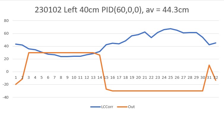
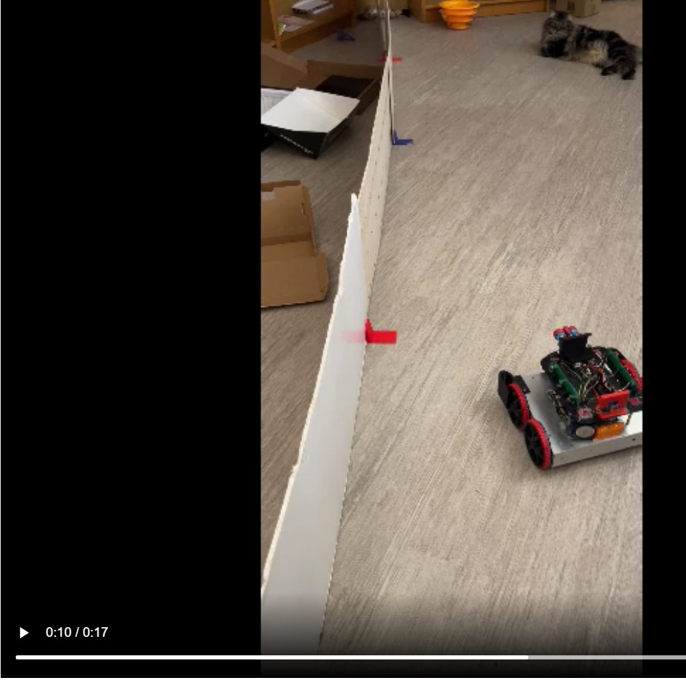
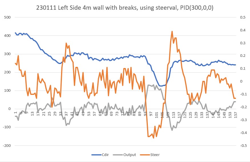
So this is the ‘other’ method – using the modified steering value as the input, and trying to drive the system to zero. Within just a few trials I rapidly homed in on one of the PID triplets I had used before, namely PID(3,0,1). Here’s the raw output, a plot of orientation-corrected distance vs setpoint, and a short video on my 4m straight wall section:
|
1 2 3 4 5 6 7 8 9 10 11 12 13 14 15 16 17 18 19 20 21 22 23 24 25 26 27 28 29 30 31 32 33 34 35 36 37 38 39 40 41 42 43 44 45 46 47 48 49 50 51 52 53 54 55 56 57 58 59 60 61 62 63 64 65 66 67 68 69 70 71 72 73 74 75 76 77 78 79 80 81 82 83 84 85 86 87 88 89 90 91 92 93 94 95 96 97 98 99 100 101 102 103 104 105 106 107 108 109 110 111 112 113 114 115 116 117 118 119 120 121 122 123 124 125 126 127 128 129 130 131 132 133 134 135 136 137 138 139 140 141 142 143 144 145 146 147 148 |
TrackLeftWallOffset: Start tracking offset of 40.0 cm with Kp/Ki/Kd = 3.00 0.00 1.00 Msec LF LC LR Steer Deg Cos LCCorr Set Err SpinDeg In TrackLeftWallOffset: before while with errcode = NO_ANOMALIES Msec LF LC LR LCCorr OffCm tErr LastI LastD Out Lspd Rspd 28916 40.10 40.30 38.80 39.21 40.00 0.79 0.00 0.79 1.58 76 73 28966 39.20 41.90 38.00 40.93 40.00 -0.93 0.00 -1.72 -1.07 73 76 29016 40.10 41.40 38.00 40.44 40.00 -0.44 0.00 0.49 -1.82 73 76 29066 40.10 41.40 37.60 37.48 40.00 2.52 0.00 2.97 4.60 79 70 29116 39.90 41.70 37.80 38.85 40.00 1.15 0.00 -1.37 4.82 79 70 29166 39.80 41.70 37.70 38.85 40.00 1.15 0.00 0.00 3.44 78 71 29216 39.60 41.10 37.90 39.23 40.00 0.77 0.00 -0.38 2.69 77 72 29266 39.90 41.80 37.90 39.20 40.00 0.80 0.00 0.03 2.38 77 72 29316 39.90 41.60 37.30 37.36 40.00 2.64 0.00 1.84 6.08 81 68 29366 40.10 42.10 37.90 38.96 40.00 1.04 0.00 -1.60 4.72 79 70 29416 40.10 41.70 38.60 40.21 40.00 -0.21 0.00 -1.25 0.62 75 74 29466 40.10 41.70 38.60 40.21 40.00 -0.21 0.00 0.00 -0.63 74 75 29516 41.10 41.80 38.90 38.68 40.00 1.32 0.00 1.53 2.43 77 72 29566 39.90 42.30 39.40 42.13 40.00 -2.13 0.00 -3.45 -2.94 72 77 29616 40.20 42.00 39.10 41.18 40.00 -1.18 0.00 0.95 -4.49 70 79 29666 40.00 42.80 38.40 41.07 40.00 -1.07 0.00 0.12 -3.31 71 78 29716 41.40 42.60 38.80 38.26 40.00 1.74 0.00 2.81 2.42 77 72 29766 40.10 41.90 38.80 40.77 40.00 -0.77 0.00 -2.51 0.21 75 74 29816 41.20 42.10 38.80 38.40 40.00 1.60 0.00 2.36 2.43 77 72 29866 41.30 42.90 38.80 39.13 40.00 0.87 0.00 -0.73 3.33 78 71 29916 41.30 42.90 38.30 37.22 40.00 2.78 0.00 1.91 6.42 81 68 29966 40.50 43.10 39.60 42.54 40.00 -2.54 0.00 -5.31 -2.30 72 77 30016 41.30 42.10 39.10 38.96 40.00 1.04 0.00 3.58 -0.46 74 75 30066 40.80 43.20 38.90 40.76 40.00 -0.76 0.00 -1.80 -0.48 74 75 30116 41.80 42.60 39.00 37.63 40.00 2.37 0.00 3.14 3.98 78 71 30166 41.20 43.00 39.90 41.84 40.00 -1.84 0.00 -4.21 -1.30 73 76 30216 41.40 43.80 38.90 39.65 40.00 0.35 0.00 2.19 -1.14 73 76 30266 41.50 44.40 38.60 38.87 40.00 1.13 0.00 0.77 2.60 77 72 30316 40.80 42.20 39.60 41.23 40.00 -1.23 0.00 -2.35 -1.32 73 76 30366 40.80 42.70 37.90 37.39 40.00 2.61 0.00 3.84 4.00 79 70 30416 40.90 43.30 39.30 41.55 40.00 -1.55 0.00 -4.16 -0.48 74 75 30466 41.30 43.50 38.30 37.74 40.00 2.26 0.00 3.80 2.97 77 72 30516 40.80 42.60 38.00 37.63 40.00 2.37 0.00 0.12 7.00 82 67 30566 40.80 42.80 38.30 38.74 40.00 1.26 0.00 -1.12 4.88 79 70 30616 40.30 42.60 38.40 40.20 40.00 -0.20 0.00 -1.45 0.86 75 74 30666 40.90 42.30 38.40 33.83 40.00 6.17 0.00 6.37 12.15 87 62 30716 41.90 44.00 39.10 38.86 40.00 1.14 0.00 -5.04 8.45 83 66 30766 41.60 44.20 40.20 42.82 40.00 -2.82 0.00 -3.96 -4.50 70 79 30816 41.50 44.00 39.20 40.43 40.00 -0.43 0.00 2.39 -3.68 71 78 30866 41.80 43.60 40.40 42.24 40.00 -2.24 0.00 -1.81 -4.91 70 79 30916 41.90 43.50 40.40 41.94 40.00 -1.94 0.00 0.29 -6.13 68 81 30966 41.70 44.40 41.40 44.33 40.00 -4.33 0.00 -2.39 -10.61 64 85 31016 41.50 44.40 40.30 43.37 40.00 -3.37 0.00 0.96 -11.08 63 86 31066 42.00 44.70 41.20 44.24 40.00 -4.24 0.00 -0.86 -11.85 63 86 31116 42.40 45.20 40.20 41.83 40.00 -1.83 0.00 2.41 -7.89 67 82 31166 42.70 44.40 40.80 41.89 40.00 -1.89 0.00 -0.07 -5.62 69 80 31216 42.40 44.90 40.20 41.55 40.00 -1.55 0.00 0.34 -5.00 70 79 31266 41.80 46.70 40.20 44.81 40.00 -4.81 0.00 -3.26 -11.17 63 86 31316 43.00 47.00 39.80 40.02 40.00 -0.02 0.00 4.79 -4.85 70 79 31366 42.80 44.90 41.30 43.29 40.00 -3.29 0.00 -3.27 -6.61 68 81 31416 42.60 46.40 40.20 42.33 40.00 -2.33 0.00 0.97 -7.95 67 82 31466 42.40 45.00 41.80 44.74 40.00 -4.74 0.00 -2.41 -11.80 63 86 31516 42.90 44.60 40.60 40.98 40.00 -0.98 0.00 3.75 -6.70 68 81 31566 43.50 45.00 40.80 40.08 40.00 -0.08 0.00 0.90 -1.15 73 76 31616 43.00 46.60 41.80 45.52 40.00 -5.52 0.00 -5.44 -11.13 63 86 31666 43.40 45.80 41.00 41.78 40.00 -1.78 0.00 3.75 -9.08 65 84 31716 43.30 45.60 40.20 39.20 40.00 0.80 0.00 2.58 -0.18 74 75 31766 42.90 45.60 41.50 44.18 40.00 -4.18 0.00 -4.97 -7.55 67 82 31816 42.80 45.70 41.60 44.64 40.00 -4.64 0.00 -0.47 -13.46 61 88 31866 43.30 46.50 41.60 44.38 40.00 -4.38 0.00 0.26 -13.41 61 88 31916 43.50 46.20 41.30 42.75 40.00 -2.75 0.00 1.63 -9.89 65 84 31966 43.70 45.80 42.70 45.79 40.00 -5.79 0.00 -3.04 -14.34 60 89 32016 43.30 46.70 42.40 46.09 40.00 -6.09 0.00 -0.30 -17.97 57 92 32066 43.40 46.40 41.70 44.29 40.00 -4.29 0.00 1.80 -14.66 60 89 32116 43.50 47.30 42.60 46.68 40.00 -6.68 0.00 -2.39 -17.65 57 92 32166 44.90 46.90 42.80 43.70 40.00 -3.70 0.00 2.98 -14.07 60 89 32216 44.70 47.10 41.70 40.87 40.00 -0.87 0.00 2.83 -5.43 69 80 32266 44.30 46.60 42.40 43.97 40.00 -3.97 0.00 -3.10 -8.81 66 83 32316 45.00 47.60 42.00 41.30 40.00 -1.30 0.00 2.67 -6.57 68 81 32366 45.20 47.30 43.20 44.36 40.00 -4.36 0.00 -3.05 -10.01 64 85 32416 44.40 48.10 43.70 47.72 40.00 -7.72 0.00 -3.36 -19.79 55 94 32466 44.50 46.90 43.90 46.63 40.00 -6.63 0.00 1.09 -20.97 54 95 32516 45.60 48.00 43.30 44.11 40.00 -4.11 0.00 2.52 -14.84 60 89 32566 45.10 47.50 43.50 45.58 40.00 -5.58 0.00 -1.47 -15.26 59 90 32616 44.60 48.00 43.30 46.70 40.00 -6.70 0.00 -1.13 -18.98 56 93 32666 45.10 48.30 43.20 45.57 40.00 -5.57 0.00 1.13 -17.85 57 92 32716 44.10 48.20 43.60 48.00 40.00 -8.00 0.00 -2.43 -21.58 53 96 32766 45.40 47.40 43.60 44.99 40.00 -4.99 0.00 3.02 -17.98 57 92 32816 44.30 47.50 43.70 47.22 40.00 -7.22 0.00 -2.23 -19.43 55 94 32866 44.80 47.90 42.80 44.92 40.00 -4.92 0.00 2.30 -17.06 57 92 32916 44.50 47.40 43.30 46.30 40.00 -6.30 0.00 -1.39 -17.53 57 92 32966 45.20 46.70 43.60 45.24 40.00 -5.24 0.00 1.06 -16.79 58 91 33016 43.60 47.40 42.10 45.71 40.00 -5.71 0.00 -0.46 -16.65 58 91 33066 44.20 47.30 42.60 45.38 40.00 -5.38 0.00 0.32 -16.47 58 91 33116 44.10 47.40 43.50 47.12 40.00 -7.12 0.00 -1.74 -19.63 55 94 33166 44.20 47.10 42.70 45.42 40.00 -5.42 0.00 1.71 -17.96 57 92 33216 43.40 47.80 42.50 47.17 40.00 -7.17 0.00 -1.76 -19.76 55 94 33266 44.50 47.20 41.60 41.33 40.00 -1.33 0.00 5.85 -9.83 65 84 33316 43.20 46.60 42.10 45.69 40.00 -5.69 0.00 -4.37 -12.71 62 87 33366 44.30 46.60 42.60 43.97 40.00 -3.97 0.00 1.72 -13.63 61 88 33416 43.80 45.80 42.50 44.56 40.00 -4.56 0.00 -0.59 -13.09 61 88 33466 43.50 46.50 42.80 46.13 40.00 -6.13 0.00 -1.57 -16.82 58 91 33516 43.50 45.80 42.60 45.20 40.00 -5.20 0.00 0.93 -16.53 58 91 33566 43.30 45.70 41.70 43.85 40.00 -3.85 0.00 1.35 -12.90 62 87 33616 42.40 46.10 42.00 45.98 40.00 -5.98 0.00 -2.13 -15.81 59 90 33666 43.10 46.00 42.00 45.10 40.00 -5.10 0.00 0.88 -16.19 58 91 33716 42.60 45.30 40.40 41.92 40.00 -1.92 0.00 3.18 -8.95 66 83 33766 42.60 45.30 40.40 41.92 40.00 -1.92 0.00 0.00 -5.76 69 80 33816 42.30 46.40 40.90 44.95 40.00 -4.95 0.00 -3.03 -11.82 63 86 33866 42.30 46.40 40.90 44.95 40.00 -4.95 0.00 0.00 -14.85 60 89 33916 42.30 44.20 41.90 44.08 40.00 -4.08 0.00 0.87 -13.12 61 88 33966 42.40 44.10 40.80 42.31 40.00 -2.31 0.00 1.77 -8.71 66 83 34016 41.50 45.50 41.10 45.43 40.00 -5.43 0.00 -3.12 -13.18 61 88 34066 41.50 44.50 41.40 44.49 40.00 -4.49 0.00 0.94 -14.42 60 89 34116 41.20 44.40 40.30 43.82 40.00 -3.82 0.00 0.67 -12.13 62 87 34166 40.70 44.10 40.40 44.04 40.00 -4.04 0.00 -0.22 -11.89 63 86 34216 40.40 43.90 39.90 43.72 40.00 -3.72 0.00 0.31 -11.48 63 86 34266 40.20 43.10 39.60 42.85 40.00 -2.85 0.00 0.87 -9.42 65 84 34316 40.00 43.10 40.00 43.10 40.00 -3.10 0.00 -0.25 -9.05 65 84 34366 40.30 43.20 39.10 42.20 40.00 -2.20 0.00 0.90 -7.50 67 82 34416 40.30 43.40 39.20 42.56 40.00 -2.56 0.00 -0.35 -7.31 67 82 34466 39.80 42.90 38.90 42.34 40.00 -2.34 0.00 0.22 -7.23 67 82 34516 39.20 42.40 37.70 40.88 40.00 -0.88 0.00 1.45 -4.11 70 79 34566 38.70 43.70 38.40 43.64 40.00 -3.64 0.00 -2.75 -8.16 66 83 34616 40.00 42.20 37.60 38.49 40.00 1.51 0.00 5.14 -0.62 74 75 34666 39.30 41.30 38.20 40.50 40.00 -0.50 0.00 -2.00 0.51 75 74 34716 38.40 42.80 37.50 42.24 40.00 -2.24 0.00 -1.74 -4.97 70 79 34766 37.90 41.80 36.90 41.13 40.00 -1.13 0.00 1.11 -4.49 70 79 34816 37.70 42.20 36.10 40.49 40.00 -0.49 0.00 0.64 -2.11 72 77 34866 37.70 41.40 36.10 39.72 40.00 0.28 0.00 0.77 0.07 75 74 34916 37.50 41.10 36.30 40.15 40.00 -0.15 0.00 -0.43 -0.02 74 75 34966 37.20 40.70 35.40 38.63 40.00 1.37 0.00 1.52 2.59 77 72 35016 37.00 39.20 37.20 39.17 40.00 0.83 0.00 -0.54 3.02 78 71 35066 37.40 40.10 34.90 36.30 40.00 3.70 0.00 2.87 8.23 83 66 35116 36.40 39.20 35.50 38.69 40.00 1.31 0.00 -2.39 6.33 81 68 35166 36.60 40.70 35.40 39.76 40.00 0.24 0.00 -1.07 1.79 76 73 35216 35.60 37.90 36.10 37.75 40.00 2.25 0.00 2.01 4.75 79 70 35266 37.10 39.80 34.30 35.15 40.00 4.85 0.00 2.59 11.95 86 63 35316 37.00 40.00 35.40 38.38 40.00 1.62 0.00 -3.23 8.09 83 66 35366 37.90 39.40 34.90 34.19 40.00 5.81 0.00 4.19 13.25 88 61 35416 37.70 41.00 34.80 35.90 40.00 4.10 0.00 -1.71 14.02 89 60 35466 37.00 41.10 35.30 39.23 40.00 0.77 0.00 -3.33 5.65 80 69 35516 37.40 40.40 35.60 38.34 40.00 1.66 0.00 0.88 4.08 79 70 35566 37.40 40.20 34.60 35.51 40.00 4.49 0.00 2.84 10.64 85 64 35616 37.40 40.20 34.60 35.51 40.00 4.49 0.00 0.00 13.48 88 61 35666 37.00 39.60 35.80 38.69 40.00 1.31 0.00 -3.18 7.12 82 67 35716 37.10 40.70 35.60 39.25 40.00 0.75 0.00 -0.56 2.82 77 72 35766 37.70 40.30 35.90 38.25 40.00 1.75 0.00 1.00 4.26 79 70 35816 37.10 40.50 34.80 37.22 40.00 2.78 0.00 1.03 7.32 82 67 35866 37.10 39.80 34.80 36.57 40.00 3.43 0.00 0.64 9.64 84 65 35916 36.80 39.50 35.60 38.59 40.00 1.41 0.00 -2.01 6.25 81 68 35966 37.20 40.70 35.00 37.66 40.00 2.34 0.00 0.92 6.08 81 68 36016 36.80 40.50 35.00 37.48 40.00 2.52 0.00 0.19 7.38 82 67 |
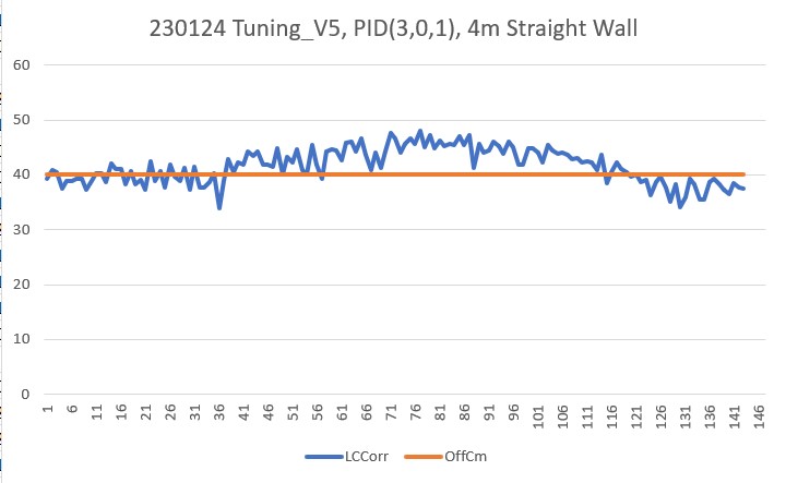
So, the ‘steering value tweaked by offset error’ method works on a straight wall with a PID of (3,0,1). This result is consistent with my 11 January 2023 Update of my ‘WallE3 Wall Tracking Revisited‘ post, which I think was done with WallE3_WallTrackTuning_V5 (too many changes for my poor brain to follow).
Unfortunately, as soon as I put breaks in the wall, the robot could no longer follow it. It runs into the same problems; the robot senses a significant change in distance, starts to turn to minimize the distance, but the distance continues to go in the wrong direction due to the change in the robot’s orientation. This feedback continues until the robot is completely orthogonal to the wall.
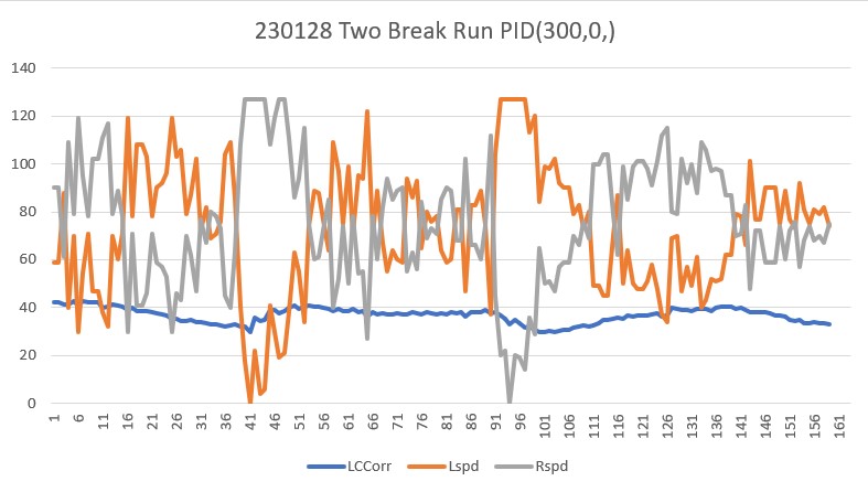
26 January 2023 Update:
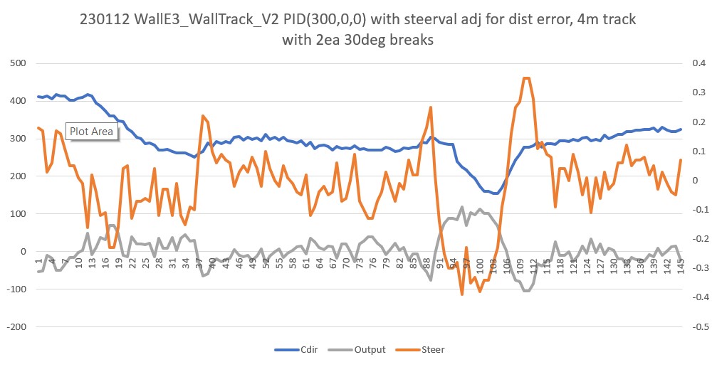
I went back and reviewed the post that contained the successful 30 October 2022 ‘two 30deg wall breaks’ run, and found that the run was made with the following wall following code:
|
1 2 3 4 5 6 7 8 9 10 11 12 13 14 15 16 17 18 19 20 21 22 23 24 25 26 27 28 29 30 31 32 33 34 35 36 37 38 |
{ digitalToggle(RED_LASER_DIODE_PIN); //10/24/22 toggle duration measurement pulse mSecSinceLastWallTrackUpdate -= WALL_TRACK_UPDATE_INTERVAL_MSEC; //03/08/22 abstracted these calls to UpdateAllEnvironmentParameters() UpdateAllEnvironmentParameters();//03/08/22 added to consolidate sensor update calls //from Teensy_7VL53L0X_I2C_Slave_V3.ino: LeftSteeringVal = (LF_Dist_mm - LR_Dist_mm) / 100.f; //rev 06/21/20 see PPalace post float orientdeg = GetWallOrientDeg(glLeftSteeringVal); float orientrad = (PI / 180.f) * orientdeg; float orientcos = cosf(orientrad); glLeftCentCorrCm = glLeftCenterCm * orientcos; if (!isnan(glLeftCentCorrCm)) { //gl_pSerPort->printf("just before PIDCalcs call: WallTrackSetPoint = %2.2f\n", WallTrackSetPoint); WallTrackOutput = PIDCalcs(glLeftCentCorrCm, WallTrackSetPoint, lastError, lastInput, lastIval, lastDerror, kp, ki, kd); //04/05/22 have to use local var here, as result could be negative int16_t leftSpdnum = MOTOR_SPEED_QTR + WallTrackOutput; int16_t rightSpdnum = MOTOR_SPEED_QTR - WallTrackOutput; //04/05/22 Left/rightSpdnum can be negative here - watch out! rightSpdnum = (rightSpdnum <= MOTOR_SPEED_HALF) ? rightSpdnum : MOTOR_SPEED_HALF; //result can still be neg glRightspeednum = (rightSpdnum > 0) ? rightSpdnum : 0; //result here must be positive leftSpdnum = (leftSpdnum <= MOTOR_SPEED_HALF) ? leftSpdnum : MOTOR_SPEED_HALF;//result can still be neg glLeftspeednum = (leftSpdnum > 0) ? leftSpdnum : 0; //result here must be positive MoveAhead(glLeftspeednum, glRightspeednum); gl_pSerPort->printf(WallFollowTelemStr, millis(), glLeftFrontCm, glLeftCenterCm, glLeftRearCm, glLeftSteeringVal, orientdeg, orientcos, glLeftCentCorrCm, WallTrackSetPoint, lastError, WallTrackOutput, glLeftspeednum, glRightspeednum); } digitalToggle(RED_LASER_DIODE_PIN); //10/24/22 toggle duration measurement pulse |
As can be seen from the above, the line
|
1 2 |
WallTrackOutput = PIDCalcs(glLeftCentCorrCm, WallTrackSetPoint, lastError, lastInput, lastIval, lastDerror, kp, ki, kd); |
Compares the orientation-corrected wall distance to the desired offset distance, as opposed to comparing the computed steering value to a desired steering value of zero, with a ‘fudge factor’ of the distance error divided by 10 as shown below:
|
1 2 3 4 |
//from Teensy_7VL53L0X_I2C_Slave_V3.ino: LeftSteeringVal = (LF_Dist_mm - LR_Dist_mm) / 100.f; //rev 06/21/20 see PPalace post glLeftCentCorrCm = CorrDistForOrient(glLeftCenterCm, glLeftSteeringVal); float offset_factor = (glLeftCentCorrCm - OffCm) / 10.f; WallTrackSteerVal = glLeftSteeringVal + offset_factor; |
So, I modified WallE3_WallTrackTuning_V5 to use the above algorithm to see if I could reproduce the successful ‘two breaks’ tracking run.
Well, the answer was “NO” – I couldn’t reproduce the successful ‘two breaks’ tracking run – not even close – grrr!!
So, as kind of a ‘Hail Mary’ move, I went back to WallE3_WallTrack_V2, which I vaguely remember as the source of the successful ‘two break’ run, and tried it without modification. Lo and Behold – IT WORKED! Whew, I was beginning to wonder if maybe (despite having a video) it was all a dream!
So, now I have a baseline – yes!!! Here’s the output and video from a successful ‘two break’ run:
|
1 2 3 4 5 6 7 8 9 10 11 12 13 14 15 16 17 18 19 20 21 22 23 24 25 26 27 28 29 30 31 32 33 34 35 36 37 38 39 40 41 42 43 44 45 46 47 48 49 50 51 52 53 54 55 56 57 58 59 60 61 62 63 64 65 66 67 68 69 70 71 72 73 74 75 76 77 78 79 80 81 82 83 84 85 86 87 88 89 90 91 92 93 94 95 96 97 98 99 100 101 102 103 104 105 106 107 108 109 110 111 112 113 114 115 116 117 118 119 120 121 122 123 124 125 126 127 128 129 130 131 132 133 134 |
TrackLeftWallOffset: Start tracking offset of 40.00cm with Kp/Ki/Kd = 300.00 0.00 0.00 Msec Fdir Cdir Rdir Steer Set error Ival Kp*err Ki*Ival Kd*Din Output Lspd Rspd 15682 405 436 405 0.04 0.00 -0.04 0.00 -10.80 0.00 -0.00 -10.80 64 85 15732 406 440 401 0.09 0.00 -0.09 0.00 -27.00 0.00 -0.00 -27.00 48 102 15782 414 437 402 0.16 0.00 -0.16 0.00 -47.10 0.00 -0.00 -47.10 27 122 15832 406 433 402 0.07 0.00 -0.07 0.00 -21.90 0.00 0.00 -21.90 53 96 15882 401 430 399 0.05 0.00 -0.05 0.00 -15.00 0.00 0.00 -15.00 60 90 15932 408 431 404 0.07 0.00 -0.07 0.00 -21.30 0.00 -0.00 -21.30 53 96 15982 406 420 408 0.00 0.00 0.00 0.00 0.00 0.00 0.00 0.00 75 75 16032 409 435 405 0.08 0.00 -0.08 0.00 -22.50 0.00 -0.00 -22.50 52 97 16082 409 435 405 0.08 0.00 -0.08 0.00 -22.50 0.00 0.00 -22.50 52 97 16132 413 427 410 0.06 0.00 -0.06 0.00 -17.10 0.00 0.00 -17.10 57 92 16182 403 426 405 0.01 0.00 -0.01 0.00 -1.80 0.00 0.00 -1.80 73 76 16232 391 425 403 -0.09 0.00 0.09 0.00 28.50 0.00 0.00 28.50 103 46 16282 397 420 399 0.00 0.00 0.00 0.00 0.00 0.00 -0.00 0.00 75 75 16332 384 415 393 -0.08 0.00 0.08 0.00 22.50 0.00 0.00 22.50 97 52 16382 381 407 392 -0.10 0.00 0.10 0.00 30.90 0.00 0.00 30.90 105 44 16432 387 401 387 0.00 0.00 -0.00 0.00 -0.30 0.00 -0.00 -0.30 74 75 16482 372 395 371 0.00 0.00 -0.00 0.00 -1.50 0.00 -0.00 -1.50 73 76 16532 372 395 371 0.00 0.00 -0.00 0.00 -1.50 0.00 0.00 -1.50 73 76 16582 364 382 372 -0.10 0.00 0.10 0.00 29.40 0.00 0.00 29.40 104 45 16632 357 387 369 -0.13 0.00 0.13 0.00 39.90 0.00 0.00 39.90 114 35 16682 351 376 362 -0.13 0.00 0.13 0.00 40.20 0.00 0.00 40.20 115 34 16732 349 370 358 -0.12 0.00 0.12 0.00 36.00 0.00 -0.00 36.00 111 39 16782 346 360 348 -0.06 0.00 0.06 0.00 18.00 0.00 -0.00 18.00 93 57 16832 344 355 344 -0.05 0.00 0.05 0.00 13.50 0.00 -0.00 13.50 88 61 16882 331 352 343 -0.17 0.00 0.17 0.00 50.40 0.00 0.00 50.40 125 24 16932 336 345 333 -0.03 0.00 0.03 0.00 7.50 0.00 -0.00 7.50 82 67 16982 326 343 339 -0.19 0.00 0.19 0.00 56.10 0.00 0.00 56.10 131 18 17032 329 337 327 -0.04 0.00 0.04 0.00 12.90 0.00 -0.00 12.90 87 62 17082 324 335 326 -0.08 0.00 0.08 0.00 25.50 0.00 0.00 25.50 100 49 17132 330 343 319 0.05 0.00 -0.05 0.00 -15.90 0.00 -0.00 -15.90 59 90 17182 341 357 319 0.18 0.00 -0.18 0.00 -53.10 0.00 -0.00 -53.10 21 128 17232 355 382 334 0.20 0.00 -0.20 0.00 -60.60 0.00 -0.00 -60.60 14 135 17282 363 394 345 0.17 0.00 -0.17 0.00 -52.20 0.00 0.00 -52.20 22 127 17332 369 394 357 0.11 0.00 -0.11 0.00 -34.20 0.00 0.00 -34.20 40 109 17382 377 398 365 0.12 0.00 -0.12 0.00 -35.40 0.00 -0.00 -35.40 39 110 17432 392 403 369 0.23 0.00 -0.23 0.00 -69.90 0.00 -0.00 -69.90 5 144 17482 384 407 367 0.18 0.00 -0.18 0.00 -53.10 0.00 0.00 -53.10 21 128 17532 389 406 375 0.15 0.00 -0.15 0.00 -43.80 0.00 0.00 -43.80 31 118 17582 382 407 375 0.08 0.00 -0.08 0.00 -23.10 0.00 0.00 -23.10 51 98 17632 383 409 383 0.01 0.00 -0.01 0.00 -2.70 0.00 0.00 -2.70 72 77 17682 381 404 384 -0.03 0.00 0.03 0.00 7.80 0.00 0.00 7.80 82 67 17732 382 408 382 0.01 0.00 -0.01 0.00 -2.40 0.00 -0.00 -2.40 72 77 17782 397 419 382 0.17 0.00 -0.17 0.00 -50.70 0.00 -0.00 -50.70 24 125 17832 393 404 380 0.13 0.00 -0.13 0.00 -40.20 0.00 0.00 -40.20 34 115 17882 389 406 387 0.03 0.00 -0.03 0.00 -7.80 0.00 0.00 -7.80 67 82 17932 396 417 390 0.08 0.00 -0.08 0.00 -23.10 0.00 -0.00 -23.10 51 98 17982 396 407 390 0.07 0.00 -0.07 0.00 -20.10 0.00 0.00 -20.10 54 95 18032 388 418 389 0.01 0.00 -0.01 0.00 -2.40 0.00 0.00 -2.40 72 77 18082 385 404 386 -0.01 0.00 0.01 0.00 1.80 0.00 0.00 1.80 76 73 18132 385 405 388 -0.02 0.00 0.02 0.00 7.50 0.00 0.00 7.50 82 67 18182 388 407 386 0.03 0.00 -0.03 0.00 -8.10 0.00 -0.00 -8.10 66 83 18232 380 399 383 -0.03 0.00 0.03 0.00 9.30 0.00 0.00 9.30 84 65 18282 383 398 383 -0.00 0.00 0.00 0.00 0.60 0.00 -0.00 0.60 75 74 18332 379 399 386 -0.07 0.00 0.07 0.00 21.30 0.00 0.00 21.30 96 53 18382 379 398 383 -0.06 0.00 0.06 0.00 18.60 0.00 -0.00 18.60 93 56 18432 381 400 381 0.00 0.00 0.00 0.00 0.00 0.00 -0.00 0.00 75 75 18482 376 395 377 -0.01 0.00 0.01 0.00 4.50 0.00 0.00 4.50 79 70 18532 377 399 375 0.02 0.00 -0.02 0.00 -5.70 0.00 -0.00 -5.70 69 80 18582 372 400 372 0.00 0.00 0.00 0.00 0.00 0.00 0.00 0.00 75 75 18632 376 399 373 -0.03 0.00 0.03 0.00 9.30 0.00 0.00 9.30 84 65 18682 374 395 376 -0.02 0.00 0.02 0.00 7.50 0.00 -0.00 7.50 82 67 18732 374 395 376 -0.02 0.00 0.02 0.00 7.50 0.00 0.00 7.50 82 67 18782 377 402 380 -0.03 0.00 0.03 0.00 8.40 0.00 0.00 8.40 83 66 18832 378 398 370 0.08 0.00 -0.08 0.00 -23.40 0.00 -0.00 -23.40 51 98 18882 377 393 377 -0.01 0.00 0.01 0.00 2.10 0.00 0.00 2.10 77 72 18932 377 393 377 -0.01 0.00 0.01 0.00 2.10 0.00 0.00 2.10 77 72 18982 381 403 371 0.10 0.00 -0.10 0.00 -30.90 0.00 -0.00 -30.90 44 105 19032 384 403 371 0.10 0.00 -0.10 0.00 -30.90 0.00 0.00 -30.90 44 105 19082 384 395 383 0.00 0.00 -0.00 0.00 -1.50 0.00 0.00 -1.50 73 76 19132 381 409 377 0.05 0.00 -0.05 0.00 -14.70 0.00 -0.00 -14.70 60 89 19182 381 395 381 -0.00 0.00 0.00 0.00 1.50 0.00 0.00 1.50 76 73 19232 384 399 377 0.07 0.00 -0.07 0.00 -20.70 0.00 -0.00 -20.70 54 95 19282 377 404 380 -0.03 0.00 0.03 0.00 7.80 0.00 0.00 7.80 82 67 19332 385 404 380 -0.03 0.00 0.03 0.00 7.80 0.00 0.00 7.80 82 67 19382 377 408 379 -0.01 0.00 0.01 0.00 3.60 0.00 -0.00 3.60 78 71 19432 381 405 380 0.01 0.00 -0.01 0.00 -4.50 0.00 -0.00 -4.50 70 79 19482 384 405 380 0.04 0.00 -0.04 0.00 -13.50 0.00 -0.00 -13.50 61 88 19532 381 407 385 -0.03 0.00 0.03 0.00 9.90 0.00 0.00 9.90 84 65 19582 384 404 381 0.03 0.00 -0.03 0.00 -10.20 0.00 -0.00 -10.20 64 85 19632 384 401 379 0.05 0.00 -0.05 0.00 -15.30 0.00 -0.00 -15.30 59 90 19682 383 404 382 0.01 0.00 -0.01 0.00 -4.20 0.00 0.00 -4.20 70 79 19732 388 410 383 0.06 0.00 -0.06 0.00 -18.00 0.00 -0.00 -18.00 57 93 19782 379 405 383 -0.04 0.00 0.04 0.00 10.50 0.00 0.00 10.50 85 64 19832 370 400 383 -0.13 0.00 0.13 0.00 39.00 0.00 0.00 39.00 114 36 19882 356 374 380 -0.27 0.00 0.27 0.00 79.80 0.00 0.00 79.80 154 0 19932 348 378 364 -0.18 0.00 0.18 0.00 54.60 0.00 -0.00 54.60 129 20 19982 331 357 353 -0.26 0.00 0.26 0.00 78.90 0.00 0.00 78.90 153 0 20032 329 340 353 -0.30 0.00 0.30 0.00 90.00 0.00 0.00 90.00 165 0 20082 324 337 345 -0.27 0.00 0.27 0.00 81.90 0.00 -0.00 81.90 156 0 20132 305 324 326 -0.29 0.00 0.29 0.00 85.80 0.00 0.00 85.80 160 0 20182 297 318 317 -0.28 0.00 0.28 0.00 84.60 0.00 -0.00 84.60 159 0 20232 299 313 302 -0.12 0.00 0.12 0.00 35.10 0.00 -0.00 35.10 110 39 20282 297 301 297 -0.10 0.00 0.10 0.00 29.70 0.00 -0.00 29.70 104 45 20332 298 303 292 -0.04 0.00 0.04 0.00 11.10 0.00 -0.00 11.10 86 63 20382 305 305 292 0.03 0.00 -0.03 0.00 -10.50 0.00 -0.00 -10.50 64 85 20432 318 322 304 0.06 0.00 -0.06 0.00 -18.60 0.00 -0.00 -18.60 56 93 20482 331 326 310 0.14 0.00 -0.14 0.00 -40.80 0.00 -0.00 -40.80 34 115 20532 331 326 310 0.14 0.00 -0.14 0.00 -40.80 0.00 0.00 -40.80 34 115 20582 335 335 319 0.09 0.00 -0.09 0.00 -28.50 0.00 0.00 -28.50 46 103 20632 339 348 321 0.13 0.00 -0.13 0.00 -38.40 0.00 -0.00 -38.40 36 113 20682 344 357 330 0.10 0.00 -0.10 0.00 -29.10 0.00 0.00 -29.10 45 104 20732 347 365 342 0.02 0.00 -0.02 0.00 -4.50 0.00 0.00 -4.50 70 79 20782 356 369 339 0.14 0.00 -0.14 0.00 -41.70 0.00 -0.00 -41.70 33 116 20832 358 370 348 0.07 0.00 -0.07 0.00 -21.00 0.00 0.00 -21.00 54 96 20882 354 378 352 -0.00 0.00 0.00 0.00 0.60 0.00 0.00 0.60 75 74 20932 359 378 352 -0.00 0.00 0.00 0.00 0.60 0.00 0.00 0.60 75 74 20982 359 385 354 0.04 0.00 -0.04 0.00 -10.50 0.00 -0.00 -10.50 64 85 21032 361 380 352 0.07 0.00 -0.07 0.00 -21.00 0.00 -0.00 -21.00 54 96 21082 361 387 360 -0.00 0.00 0.00 0.00 0.90 0.00 0.00 0.90 75 74 21132 371 384 360 0.09 0.00 -0.09 0.00 -28.20 0.00 -0.00 -28.20 46 103 21182 375 399 369 0.06 0.00 -0.06 0.00 -17.70 0.00 0.00 -17.70 57 92 21232 381 404 381 0.00 0.00 -0.00 0.00 -1.20 0.00 0.00 -1.20 73 76 21282 379 403 373 0.06 0.00 -0.06 0.00 -18.90 0.00 -0.00 -18.90 56 93 21332 390 403 371 0.19 0.00 -0.19 0.00 -57.90 0.00 -0.00 -57.90 17 132 21382 394 400 379 0.15 0.00 -0.15 0.00 -45.00 0.00 0.00 -45.00 30 120 21432 394 405 385 0.10 0.00 -0.10 0.00 -28.50 0.00 0.00 -28.50 46 103 21482 391 417 386 0.07 0.00 -0.07 0.00 -20.10 0.00 0.00 -20.10 54 95 21532 390 420 389 0.03 0.00 -0.03 0.00 -9.00 0.00 0.00 -9.00 66 84 21582 397 415 387 0.12 0.00 -0.12 0.00 -34.50 0.00 -0.00 -34.50 40 109 21632 397 414 396 0.02 0.00 -0.02 0.00 -7.20 0.00 0.00 -7.20 67 82 21682 396 416 388 0.10 0.00 -0.10 0.00 -28.80 0.00 -0.00 -28.80 46 103 21732 403 422 397 0.08 0.00 -0.08 0.00 -24.60 0.00 0.00 -24.60 50 99 21782 407 423 401 0.08 0.00 -0.08 0.00 -24.90 0.00 -0.00 -24.90 50 99 21832 402 427 402 0.03 0.00 -0.03 0.00 -8.10 0.00 0.00 -8.10 66 83 21882 397 434 392 0.08 0.00 -0.08 0.00 -25.20 0.00 -0.00 -25.20 49 100 21932 409 429 399 0.13 0.00 -0.13 0.00 -38.70 0.00 -0.00 -38.70 36 113 21982 408 430 414 -0.03 0.00 0.03 0.00 9.00 0.00 0.00 9.00 84 66 22032 403 428 400 0.06 0.00 -0.06 0.00 -17.40 0.00 -0.00 -17.40 57 92 22082 403 428 400 0.06 0.00 -0.06 0.00 -17.40 0.00 0.00 -17.40 57 92 22132 401 424 403 0.00 0.00 -0.00 0.00 -1.20 0.00 0.00 -1.20 73 76 22182 402 421 406 -0.02 0.00 0.02 0.00 5.70 0.00 0.00 5.70 80 69 22232 400 421 402 0.00 0.00 -0.00 0.00 -0.30 0.00 -0.00 -0.30 74 75 |
And here is the wall tracking code for this run:
|
1 2 3 4 5 6 7 8 9 10 11 12 13 14 15 16 17 18 19 20 21 22 23 24 25 26 27 28 29 30 31 32 33 34 35 36 37 38 39 40 41 42 43 44 45 46 47 48 49 50 51 52 53 54 55 56 57 58 59 60 61 62 63 64 65 66 67 68 69 70 71 72 73 74 75 76 77 78 79 80 81 82 83 84 85 86 87 88 89 90 91 92 93 94 95 96 97 98 99 100 101 102 103 104 105 106 107 108 109 110 111 112 113 114 115 116 117 118 119 120 121 122 123 124 125 126 127 128 129 130 131 132 133 134 135 136 137 138 139 140 141 142 143 144 145 146 147 148 149 150 151 152 153 154 155 156 157 158 159 160 161 162 163 164 165 166 167 168 169 170 171 172 173 174 175 176 177 178 179 |
void TrackLeftWallOffset(float kp, float ki, float kd, float offsetCm) { //Notes: // 06/21/21 modified to do a turn, then straight, then track 0 steer val mSecSinceLastWallTrackUpdate = 0; float lastError = 0; float lastInput = 0; float lastIval = 0; float lastDerror = 0; float spinRateDPS = 30; GetRequestedVL53l0xValues(VL53L0X_LEFT); //update glLeftSteeringVal myTeePrint.printf("\nIn TrackLeftWallOffset with Kp/Ki/Kd = %2.2f\t%2.2f\t%2.2f\n", kp, ki, kd); //06/21/21 modified to do a turn, then straight, then track 0 steer val float cutAngleDeg = WALL_OFFSET_TGTDIST_CM - (int)(glLidar_LeftCenter / 10.f);//positive inside, negative outside desired offset myTeePrint.printf("R/C/F dists = %d\t%d\t%d Steerval = %2.3f, CutAngle = %2.2f\n", glLidar_LeftRear, glLidar_LeftCenter, glLidar_LeftFront, glLeftSteeringVal, cutAngleDeg); //07/05/21 implement min cut angle if (cutAngleDeg < 0 && abs(cutAngleDeg) < WALL_OFFSET_APPR_ANGLE_MINDEG) { myTeePrint.printf("(cutAngleDeg < 0 && abs(cutAngleDeg) < %d -- setting to -%d\n", WALL_OFFSET_APPR_ANGLE_MINDEG, WALL_OFFSET_APPR_ANGLE_MINDEG); cutAngleDeg = -WALL_OFFSET_APPR_ANGLE_MINDEG; } else if (cutAngleDeg > 0 && cutAngleDeg < WALL_OFFSET_APPR_ANGLE_MINDEG) { myTeePrint.printf("(cutAngleDeg > 0 && abs(cutAngleDeg) < %d -- setting to +%d\n", WALL_OFFSET_APPR_ANGLE_MINDEG, WALL_OFFSET_APPR_ANGLE_MINDEG); cutAngleDeg = WALL_OFFSET_APPR_ANGLE_MINDEG; } //get the steering angle from the steering value, for comparison to the computed cut angle //positive value means robot is oriented away from wall float SteerAngleDeg = GetSteeringAngle(glLeftSteeringVal); GetRequestedVL53l0xValues(VL53L0X_LEFT); myTeePrint.printf("R/C/F dists = %d\t%d\t%d Steerval = %2.3f, SteerAngle = %2.2f, CutAngle = %2.2f\n", glLidar_LeftRear, glLidar_LeftCenter, glLidar_LeftFront, glLeftSteeringVal, SteerAngleDeg, cutAngleDeg); //now decide which way to turn. int16_t fudgeFactorMM = 0; //07/05/21 added so can change for inside vs outside starting condx if (cutAngleDeg > 0) //robot inside desired offset distance { if (SteerAngleDeg > cutAngleDeg) // --> SteerAngleDeg also > 0, have to turn CCW { myTeePrint.printf("CutAngDeg > 0, SteerAngleDeg > cutAngleDeg - Turn CCW to cut angle\n"); SpinTurn(true, SteerAngleDeg - cutAngleDeg, spinRateDPS); // } else //(SteerAngleDeg <= cutAngleDeg)// --> SteerAngleDeg could be < 0 { myTeePrint.printf("CutAngDeg > 0, SteerAngleDeg < cutAngleDeg\n"); SpinTurn(false, cutAngleDeg - SteerAngleDeg, spinRateDPS); //turn diff between SteerAngleDeg & cutAngleDeg } fudgeFactorMM = -100; //07/05/21 don't need fudge factor for inside start condx } else // cutAngleDeg < 0 --> robot outside desired offset distance { if (SteerAngleDeg > cutAngleDeg) // --> SteerAngleDeg may also be > 0 { //robot turned too far toward wall myTeePrint.printf("CutAngDeg < 0, SteerAngleDeg > cutAngleDeg\n"); SpinTurn(true, SteerAngleDeg - cutAngleDeg, spinRateDPS); // } else// (SteerAngleDeg < cutAngleDeg)// --> SteerAngleDeg must also be < 0 { //robot turned to far away from wall myTeePrint.printf("CutAngDeg < 0, SteerAngleDeg <= 0\n"); SpinTurn(false, cutAngleDeg - SteerAngleDeg, spinRateDPS); //null out SteerAngleDeg & then turn addnl cutAngleDeg } fudgeFactorMM = 100; //07/05/21 need fudge factor for outside start condx } myTeePrint.printf("fudgeFactorMM = %d\n", fudgeFactorMM); delay(1000); //adjust so offset capture occurs at correct perpendicular offset float adjfactor = cos(PI * cutAngleDeg / 180.f); float numerator = 10 * (float)WALL_OFFSET_TGTDIST_CM; float adjOffsetMM = (numerator / adjfactor); adjOffsetMM += fudgeFactorMM; //fudge factor for distance measurements lagging behind robot's travel. myTeePrint.printf("\nat approach start: cut angle = %2.3f, adjfactor = %2.3f, num = %2.2f, tgt dist = %2.2f\n", cutAngleDeg, adjfactor, numerator, adjOffsetMM); GetRequestedVL53l0xValues(VL53L0X_ALL); //added 09/05/21 long int err = glLidar_LeftFront - adjOffsetMM; //neg for inside going out, pos for outside going in long int prev_err = err; myTeePrint.printf("At start - err = prev_err = %ld\n", err, prev_err); SteerAngleDeg = GetSteeringAngle(glLeftSteeringVal); myTeePrint.printf("R/C/F dists = %d\t%d\t%d Steerval = %2.3f, SteerAngle = %2.2f, CutAngle = %2.2f, err/prev_err = %li\n", glLidar_LeftRear, glLidar_LeftCenter, glLidar_LeftFront, glLeftSteeringVal, SteerAngleDeg, cutAngleDeg, err); myTeePrint.printf("Msec\tLFront\tLCtr\tLRear\tFront\tRear\tErr\tP_err\n"); //TIMSK5 = 0; //turn off TIMER5 interrupts //09/05/21 rev to doublecheck robot position - might not need the forward motion section while (((cutAngleDeg > 0 && err < 0) || (cutAngleDeg <= 0 && err >= 0)) && prev_err * err > 0) //sign change makes this < 0 { prev_err = err; //MoveAhead(MOTOR_SPEED_QTR, MOTOR_SPEED_QTR); MoveAhead(MOTOR_SPEED_FULL, MOTOR_SPEED_FULL); delay(100); glFrontdistval = GetFrontDistCm(); GetRequestedVL53l0xValues(VL53L0X_ALL); err = glLidar_LeftFront - adjOffsetMM; //06/29/21 now adj for slant dist vs perp dist myTeePrint.printf("%lu\t%d\t%d\t%d\t%d\t%d\t%ld\t%ld\n", millis(), glLidar_LeftFront, glLidar_LeftCenter, glLidar_LeftRear, glFrontdistval, glLidar_Rear, err, prev_err); CheckForUserInput(); } //now turn back the same (unadjusted) amount myTeePrint.printf("At end of offset capture - prev_res*res = %ld\n", prev_err * err); myTeePrint.printf("correct back to parallel\n"); SpinTurn(!(cutAngleDeg < 0), abs(cutAngleDeg), spinRateDPS); //have to use abs() here, as cutAngleDeg can be neg WallTrackSetPoint = 0; //moved here 6/22/21 //TIMSK5 |= (1 << OCIE5A);// enable timer compare interrupt myTeePrint.printf("\nTrackLeftWallOffset: Start tracking offset of %2.2fcm with Kp/Ki/Kd = %2.2f\t%2.2f\t%2.2f\n", offsetCm, kp, ki, kd); myTeePrint.printf("Msec\tFdir\tCdir\tRdir\tSteer\tSet\terror\tIval\tKp*err\tKi*Ival\tKd*Din\tOutput\tLspd\tRspd\n"); mSecSinceLastWallTrackUpdate = 0; //added 09/04/21 while (true) { CheckForUserInput(); //this is a bit recursive, but should still work (I hope) //now using TIMER5 100 mSec interrupt for timing //if (bTimeForNavUpdate) //{ // //mSecSinceLastWallTrackUpdate -= WALL_TRACK_UPDATE_INTERVAL_MSEC; // bTimeForNavUpdate = false; //09/04/21 back to elapsedMillis timing if (mSecSinceLastWallTrackUpdate > WALL_TRACK_UPDATE_INTERVAL_MSEC) { mSecSinceLastWallTrackUpdate -= WALL_TRACK_UPDATE_INTERVAL_MSEC; GetRequestedVL53l0xValues(VL53L0X_LEFT); //now done in TIMER5 ISR //have to weight value by both angle and wall offset WallTrackSteerVal = glLeftSteeringVal + (glLidar_LeftCenter - 10 * WALL_OFFSET_TGTDIST_CM) / 1000.f; //update motor speeds, skipping bad values if (!isnan(WallTrackSteerVal)) { //02/05/22 sampleTime removed from signature WallTrackOutput = PIDCalcs(WallTrackSteerVal, WallTrackSetPoint, lastError, lastInput, lastIval, lastDerror, kp, ki, kd); int glLeftspeednum = MOTOR_SPEED_QTR + WallTrackOutput; int glRightspeednum = MOTOR_SPEED_QTR - WallTrackOutput; glRightspeednum = (glRightspeednum <= MOTOR_SPEED_FULL) ? glRightspeednum : MOTOR_SPEED_FULL; glRightspeednum = (glRightspeednum > 0) ? glRightspeednum : 0; glLeftspeednum = (glLeftspeednum <= MOTOR_SPEED_FULL) ? glLeftspeednum : MOTOR_SPEED_FULL; glLeftspeednum = (glLeftspeednum > 0) ? glLeftspeednum : 0; MoveAhead(glLeftspeednum, glRightspeednum); myTeePrint.printf("%lu \t%d\t%d\t%d \t%2.2f\t%2.2f\t%2.2f\t%2.2f \t%2.2f\t%2.2f\t%2.2f \t%2.2f\t%d\t%d\n", millis(), glLidar_LeftFront, glLidar_LeftCenter, glLidar_LeftRear, WallTrackSteerVal, WallTrackSetPoint, lastError, lastIval, kp * lastError, ki * lastIval, kd * lastDerror, WallTrackOutput, glLeftspeednum, glRightspeednum); } } } } |
And here is just the wall tracking portion of the above function:
|
1 2 3 4 5 6 7 8 9 10 11 12 13 14 15 16 17 18 19 20 21 22 23 24 25 26 27 28 29 30 31 32 33 34 35 36 37 38 39 40 41 42 43 44 45 46 47 48 49 50 51 52 53 54 |
WallTrackSetPoint = 0; //moved here 6/22/21 //TIMSK5 |= (1 << OCIE5A);// enable timer compare interrupt myTeePrint.printf("\nTrackLeftWallOffset: Start tracking offset of %2.2fcm with Kp/Ki/Kd = %2.2f\t%2.2f\t%2.2f\n", offsetCm, kp, ki, kd); myTeePrint.printf("Msec\tFdir\tCdir\tRdir\tSteer\tSet\terror\tIval\tKp*err\tKi*Ival\tKd*Din\tOutput\tLspd\tRspd\n"); mSecSinceLastWallTrackUpdate = 0; //added 09/04/21 while (true) { CheckForUserInput(); //this is a bit recursive, but should still work (I hope) //now using TIMER5 100 mSec interrupt for timing //if (bTimeForNavUpdate) //{ // //mSecSinceLastWallTrackUpdate -= WALL_TRACK_UPDATE_INTERVAL_MSEC; // bTimeForNavUpdate = false; //09/04/21 back to elapsedMillis timing if (mSecSinceLastWallTrackUpdate > WALL_TRACK_UPDATE_INTERVAL_MSEC) { mSecSinceLastWallTrackUpdate -= WALL_TRACK_UPDATE_INTERVAL_MSEC; GetRequestedVL53l0xValues(VL53L0X_LEFT); //now done in TIMER5 ISR //have to weight value by both angle and wall offset WallTrackSteerVal = glLeftSteeringVal + (glLidar_LeftCenter - 10 * WALL_OFFSET_TGTDIST_CM) / 1000.f; //update motor speeds, skipping bad values if (!isnan(WallTrackSteerVal)) { //02/05/22 sampleTime removed from signature WallTrackOutput = PIDCalcs(WallTrackSteerVal, WallTrackSetPoint, lastError, lastInput, lastIval, lastDerror, kp, ki, kd); int glLeftspeednum = MOTOR_SPEED_QTR + WallTrackOutput; int glRightspeednum = MOTOR_SPEED_QTR - WallTrackOutput; glRightspeednum = (glRightspeednum <= MOTOR_SPEED_FULL) ? glRightspeednum : MOTOR_SPEED_FULL; glRightspeednum = (glRightspeednum > 0) ? glRightspeednum : 0; glLeftspeednum = (glLeftspeednum <= MOTOR_SPEED_FULL) ? glLeftspeednum : MOTOR_SPEED_FULL; glLeftspeednum = (glLeftspeednum > 0) ? glLeftspeednum : 0; MoveAhead(glLeftspeednum, glRightspeednum); myTeePrint.printf("%lu \t%d\t%d\t%d \t%2.2f\t%2.2f\t%2.2f\t%2.2f \t%2.2f\t%2.2f\t%2.2f \t%2.2f\t%d\t%d\n", millis(), glLidar_LeftFront, glLidar_LeftCenter, glLidar_LeftRear, WallTrackSteerVal, WallTrackSetPoint, lastError, lastIval, kp * lastError, ki * lastIval, kd * lastDerror, WallTrackOutput, glLeftspeednum, glRightspeednum); } } } |
From the above, it appears that WallE3_WallTrack_V2 uses a ‘steering value’ setpoint of zero, and also ‘tweaks’ the input to the PID engine using the error between the measured wall distance and the desired wall offset, as shown in the following snippet:
|
1 2 3 4 5 6 7 8 9 10 |
//have to weight value by both angle and wall offset WallTrackSteerVal = glLeftSteeringVal + (glLidar_LeftCenter - 10 * WALL_OFFSET_TGTDIST_CM) / 1000.f; //update motor speeds, skipping bad values if (!isnan(WallTrackSteerVal)) { //02/05/22 sampleTime removed from signature WallTrackOutput = PIDCalcs(WallTrackSteerVal, WallTrackSetPoint, lastError, lastInput, lastIval, lastDerror, kp, ki, kd); |
This is very similar to what I was trying to do in WallE3_WallTrackTuning_V5 initially below (copied here from ’24 January 2023 Update:’ above for convenience):
|
1 2 3 4 |
//from Teensy_7VL53L0X_I2C_Slave_V3.ino: LeftSteeringVal = (LF_Dist_mm - LR_Dist_mm) / 100.f; //rev 06/21/20 see PPalace post glLeftCentCorrCm = CorrDistForOrient(glLeftCenterCm, glLeftSteeringVal); float offset_factor = (glLeftCentCorrCm - OffCm) / 10.f; WallTrackSteerVal = glLeftSteeringVal + offset_factor; |
So, the original Tuning_V5 math appears to be identical to the WallTrack_V2 math; both use an offset factor as shown:
WallE3_WallTrackTuning_V5:
|
1 2 |
float offset_factor = (glLeftCentCorrCm - OffCm) / 10.f; WallTrackSteerVal = glLeftSteeringVal + offset_factor; |
WallE3_WallTrack_V2:
|
1 |
WallTrackSteerVal = glLeftSteeringVal + (glLidar_LeftCenter - 10 * WALL_OFFSET_TGTDIST_CM) / 1000.f; |
Aha! In WallE3_WallTrack_V2 the offset error (in mm) is divided by 1000, but in WallE3_WallTrackTuning_V5 the offset error (in cm) is divided by 10, which still leaves a factor of 10 difference between the two algorithms! I should be dividing the cm offset by 100 – not 10!
28 January 2023 Update:
SUCCESS!!! So I went back to my WallE3_WallTrackTuning_V5 program, and modified it to be the same as WallE3_WallTrack_V2, except using distances in cm instead of mm, and dividing by 100 instead of 10. After the usual number of stupid errors, I got the following successful run on the ‘two break’ wall setup:
|
1 2 3 4 5 6 7 8 9 10 11 12 13 14 15 16 17 18 19 20 21 22 23 24 25 26 27 28 29 30 31 32 33 34 35 36 37 38 39 40 41 42 43 44 45 46 47 48 49 50 51 52 53 54 55 56 57 58 59 60 61 62 63 64 65 66 67 68 69 70 71 72 73 74 75 76 77 78 79 80 81 82 83 84 85 86 87 88 89 90 91 92 93 94 95 96 97 98 99 100 101 102 103 104 105 106 107 108 109 110 111 112 113 114 115 116 117 118 119 120 121 122 123 124 125 126 127 128 129 130 131 132 133 134 135 136 137 138 139 140 141 142 143 144 145 146 147 148 149 150 151 152 153 154 155 156 157 158 159 160 161 162 163 164 |
WallE3_WallTrackTuning_V5.ino: TrackLeftWallOffset: Start tracking offset of 40.0 cm with Kp/Ki/Kd = 300.00 0.00 0.00 Msec LF LC LR Steer Deg Cos LCCorr Set Err SpinDeg WallE3_WallTrackTuning_V5.ino: In TrackLeftWallOffset: before while with errcode = NO_ANOMALIES Msec LF LC LR LCCorr OffCm tErr LastI LastD Out Lspd Rspd 44127 39.60 42.20 39.30 42.14 40.00 -0.05 0.00 -0.05 -15.41 59 90 44177 39.60 42.20 39.30 42.14 40.00 -0.05 0.00 0.00 -15.41 59 90 44227 39.30 41.70 39.90 41.46 40.00 0.05 0.00 0.10 13.63 88 61 44277 40.50 42.10 39.50 41.42 40.00 -0.11 0.00 -0.16 -34.26 40 109 44327 39.50 42.60 39.60 42.59 40.00 -0.02 0.00 0.10 -4.78 70 79 44377 40.30 42.20 38.90 40.88 40.00 -0.15 0.00 -0.13 -44.64 30 119 44427 40.10 42.80 39.70 42.69 40.00 -0.07 0.00 0.08 -20.07 54 95 44477 39.50 42.30 39.60 42.29 40.00 -0.01 0.00 0.05 -3.88 71 78 44527 39.90 42.60 39.20 42.26 40.00 -0.09 0.00 -0.08 -27.78 47 102 44577 40.10 42.60 39.20 42.26 40.00 -0.09 0.00 0.00 -27.78 47 102 44627 40.10 41.10 38.90 40.15 40.00 -0.12 0.00 -0.03 -36.45 38 111 44677 40.30 41.50 38.90 40.20 40.00 -0.14 0.00 -0.02 -42.61 32 117 44727 39.20 41.40 39.20 41.40 40.00 -0.01 0.00 0.13 -4.20 70 79 44777 38.70 40.90 38.30 40.79 40.00 -0.05 0.00 -0.03 -14.38 60 89 44827 38.40 40.30 38.30 40.29 40.00 -0.01 0.00 0.03 -3.88 71 78 44877 37.90 40.30 39.30 39.04 40.00 0.15 0.00 0.16 44.88 119 30 44927 37.90 40.00 38.00 39.99 40.00 0.01 0.00 -0.14 3.02 78 71 44977 37.30 39.40 38.30 38.76 40.00 0.11 0.00 0.10 33.71 108 41 45027 37.30 39.40 38.30 38.76 40.00 0.11 0.00 0.00 33.71 108 41 45077 35.90 38.90 36.70 38.50 40.00 0.10 0.00 -0.02 28.51 103 46 45127 36.60 38.00 36.50 37.99 40.00 0.01 0.00 -0.08 3.02 78 71 45177 35.60 37.90 35.90 37.84 40.00 0.05 0.00 0.04 15.47 90 59 45227 35.30 37.30 35.60 37.25 40.00 0.06 0.00 0.01 17.26 92 57 45277 34.70 36.80 35.10 36.70 40.00 0.07 0.00 0.02 21.89 96 53 45327 34.20 35.80 35.20 35.22 40.00 0.15 0.00 0.07 44.33 119 30 45377 34.00 35.60 34.50 35.46 40.00 0.10 0.00 -0.05 28.63 103 46 45427 33.60 34.50 34.50 34.36 40.00 0.11 0.00 0.01 31.92 106 43 45477 33.60 34.50 33.20 34.41 40.00 0.02 0.00 -0.09 4.77 79 70 45527 33.80 34.90 33.70 34.89 40.00 0.04 0.00 0.03 12.32 87 62 45577 32.90 34.00 33.20 33.95 40.00 0.09 0.00 0.05 27.15 102 47 45627 33.20 34.20 32.50 33.93 40.00 -0.01 0.00 -0.10 -2.78 72 77 45677 32.80 33.70 32.40 33.61 40.00 0.02 0.00 0.03 7.16 82 67 45727 33.00 33.40 32.10 32.96 40.00 -0.02 0.00 -0.04 -5.89 69 80 45777 32.60 33.40 31.80 33.05 40.00 -0.01 0.00 0.01 -3.16 71 78 45827 32.60 32.90 31.90 32.64 40.00 0.00 0.00 0.01 1.09 76 73 45877 31.90 32.20 32.10 32.18 40.00 0.10 0.00 0.09 29.46 104 45 45927 31.70 32.60 32.10 32.51 40.00 0.11 0.00 0.02 34.46 109 40 45977 32.40 33.20 32.10 33.15 40.00 0.04 0.00 -0.08 11.55 86 63 46027 33.30 34.10 31.40 32.18 40.00 -0.11 0.00 -0.15 -33.53 41 108 46077 34.80 35.80 32.10 31.89 40.00 -0.19 0.00 -0.08 -56.67 18 127 46127 36.70 37.50 32.90 29.99 40.00 -0.28 0.00 -0.09 -83.96 0 127 46177 37.00 38.50 34.80 35.63 40.00 -0.18 0.00 0.10 -52.89 22 127 46227 37.80 39.40 34.90 34.50 40.00 -0.23 0.00 -0.06 -70.49 4 127 46277 38.60 39.60 35.80 34.98 40.00 -0.23 0.00 0.01 -68.93 6 127 46327 37.70 40.00 36.50 39.08 40.00 -0.11 0.00 0.12 -33.23 41 108 46377 37.60 40.50 36.00 38.86 40.00 -0.15 0.00 -0.04 -44.58 30 119 46427 38.60 40.40 36.50 37.64 40.00 -0.19 0.00 -0.04 -55.92 19 127 46477 38.90 41.00 37.00 38.69 40.00 -0.18 0.00 0.01 -53.06 21 127 46527 38.90 41.10 37.70 40.15 40.00 -0.12 0.00 0.06 -36.45 38 111 46577 38.40 40.90 38.10 40.84 40.00 -0.04 0.00 0.08 -11.52 63 86 46627 39.00 39.70 38.30 39.38 40.00 -0.06 0.00 -0.03 -19.15 55 94 46677 39.80 41.60 38.50 40.48 40.00 -0.13 0.00 -0.07 -40.43 34 115 46727 39.10 41.10 39.20 41.09 40.00 -0.00 0.00 0.13 -0.28 74 75 46777 38.30 40.40 38.80 40.24 40.00 0.05 0.00 0.05 14.29 89 60 46827 38.40 40.80 38.90 40.63 40.00 0.04 0.00 -0.00 13.10 88 61 46877 38.90 40.10 39.00 40.09 40.00 0.01 0.00 -0.03 2.72 77 72 46927 38.20 39.60 38.30 39.50 40.00 -0.03 0.00 -0.04 -10.49 64 85 46977 37.60 39.20 38.60 38.57 40.00 0.11 0.00 0.15 34.30 109 40 47027 37.10 39.80 37.80 39.48 40.00 0.08 0.00 -0.04 22.55 97 52 47077 37.00 38.80 36.90 38.79 40.00 0.00 0.00 -0.07 0.62 75 74 47127 36.50 39.10 37.20 38.79 40.00 0.08 0.00 0.08 24.63 99 50 47177 37.70 39.30 37.50 39.27 40.00 -0.01 0.00 -0.09 -3.82 71 78 47227 36.60 38.20 37.10 38.04 40.00 0.07 0.00 0.08 20.87 95 54 47277 36.70 38.70 37.00 38.54 40.00 0.06 0.00 -0.00 19.37 94 55 47327 36.40 37.10 37.60 36.24 40.00 0.16 0.00 0.09 47.27 122 27 47377 37.00 38.20 36.70 38.14 40.00 -0.01 0.00 -0.17 -3.43 71 78 47427 36.70 37.30 36.90 37.28 40.00 0.05 0.00 0.06 14.17 89 60 47477 37.00 37.60 36.50 37.45 40.00 -0.02 0.00 -0.07 -7.34 67 82 47527 36.90 37.90 36.00 37.40 40.00 -0.06 0.00 -0.04 -19.21 55 94 47577 36.50 37.60 35.90 37.38 40.00 -0.03 0.00 0.03 -10.14 64 85 47627 36.50 38.10 35.80 37.80 40.00 -0.05 0.00 -0.01 -14.39 60 89 47677 36.60 37.50 35.80 37.11 40.00 -0.05 0.00 -0.00 -15.33 59 90 47727 36.00 37.50 36.40 37.40 40.00 0.07 0.00 0.12 19.79 94 55 47777 36.10 38.30 36.30 38.27 40.00 0.04 0.00 -0.03 11.18 86 63 47827 36.10 37.80 36.50 37.70 40.00 0.06 0.00 0.03 18.90 93 56 47877 36.40 37.40 35.80 37.18 40.00 -0.03 0.00 -0.09 -9.54 65 84 47927 35.90 38.20 35.90 38.20 40.00 0.02 0.00 0.05 5.40 80 69 47977 36.40 37.60 36.20 37.58 40.00 0.00 0.00 -0.01 1.27 76 73 48027 35.90 37.00 35.70 36.98 40.00 0.01 0.00 0.01 3.07 78 71 48077 37.00 37.80 36.40 37.58 40.00 -0.04 0.00 -0.05 -10.74 64 85 48127 36.60 37.40 35.80 37.01 40.00 -0.05 0.00 -0.01 -15.04 59 90 48177 36.50 38.20 35.80 37.90 40.00 -0.05 0.00 0.00 -14.69 60 89 48227 36.30 37.80 36.30 37.80 40.00 0.02 0.00 0.07 6.60 81 68 48277 36.50 37.90 36.50 37.90 40.00 0.02 0.00 -0.00 6.30 81 68 48327 37.20 37.30 35.90 36.29 40.00 -0.09 0.00 -0.11 -27.88 47 102 48377 37.00 38.30 37.10 38.29 40.00 0.03 0.00 0.12 8.12 83 66 48427 36.70 38.10 36.10 38.09 40.00 0.03 0.00 0.00 8.72 83 66 48477 36.20 38.10 36.50 38.04 40.00 0.05 0.00 0.02 14.87 89 60 48527 37.00 39.00 36.90 38.99 40.00 0.00 0.00 -0.05 0.02 75 74 48577 37.50 38.90 36.00 37.51 40.00 -0.13 0.00 -0.13 -37.53 37 112 48627 36.40 38.60 37.20 38.20 40.00 0.10 0.00 0.22 29.40 104 45 48677 35.50 38.10 37.00 36.74 40.00 0.18 0.00 0.08 54.79 127 20 48727 35.70 36.40 37.00 35.42 40.00 0.18 0.00 -0.01 52.75 127 22 48777 34.00 36.30 36.50 32.86 40.00 0.32 0.00 0.15 96.42 127 0 48827 34.30 35.80 35.60 34.83 40.00 0.18 0.00 -0.14 54.50 127 20 48877 33.10 34.20 34.30 33.41 40.00 0.19 0.00 0.00 55.77 127 19 48927 31.70 32.60 32.90 31.85 40.00 0.20 0.00 0.02 60.46 127 14 48977 31.30 32.20 31.80 32.07 40.00 0.13 0.00 -0.07 38.79 113 36 49027 30.50 30.90 31.10 30.72 40.00 0.15 0.00 0.02 45.84 120 29 49077 30.70 30.10 30.00 29.86 40.00 0.03 0.00 -0.12 9.42 84 65 49127 30.20 29.80 30.00 29.78 40.00 0.08 0.00 0.05 24.66 99 50 49177 30.00 30.20 29.80 30.18 40.00 0.08 0.00 -0.00 23.46 98 51 49227 30.10 29.70 30.00 29.70 40.00 0.09 0.00 0.01 27.91 102 47 49277 30.20 30.30 29.80 30.22 40.00 0.06 0.00 -0.04 17.34 92 57 49327 30.60 31.00 29.80 30.92 40.00 0.05 0.00 -0.01 15.24 90 59 49377 30.60 31.00 30.20 30.92 40.00 0.05 0.00 0.00 15.24 90 59 49427 31.50 31.70 30.80 31.45 40.00 0.02 0.00 -0.04 4.66 79 70 49477 31.40 32.30 30.90 32.17 40.00 0.03 0.00 0.01 8.49 83 66 49527 32.30 33.00 31.50 32.66 40.00 -0.01 0.00 -0.03 -1.97 73 76 49577 32.10 32.20 31.50 32.01 40.00 0.02 0.00 0.03 5.97 80 69 49627 33.60 33.90 32.00 32.53 40.00 -0.09 0.00 -0.11 -25.58 49 100 49677 34.00 34.60 32.50 33.36 40.00 -0.08 0.00 0.00 -25.09 49 100 49727 34.30 36.10 32.80 34.81 40.00 -0.10 0.00 -0.01 -29.43 45 104 49777 34.30 36.10 32.80 34.81 40.00 -0.10 0.00 0.00 -29.43 45 104 49827 34.70 35.60 34.10 35.39 40.00 -0.01 0.00 0.08 -4.17 70 79 49877 34.60 35.90 34.60 35.90 40.00 0.04 0.00 0.05 12.30 87 62 49927 35.50 36.30 34.20 35.32 40.00 -0.08 0.00 -0.12 -24.96 50 99 49977 35.90 36.80 35.20 36.51 40.00 -0.04 0.00 0.05 -10.52 64 85 50027 36.40 37.00 35.20 36.15 40.00 -0.08 0.00 -0.05 -24.44 50 99 50077 36.30 37.80 35.10 36.93 40.00 -0.09 0.00 -0.01 -26.78 48 101 50127 36.60 37.80 35.40 36.93 40.00 -0.09 0.00 0.00 -26.78 48 101 50177 37.40 37.60 36.30 36.87 40.00 -0.08 0.00 0.01 -23.60 51 98 50227 37.30 37.80 36.50 37.41 40.00 -0.05 0.00 0.02 -16.22 58 91 50277 37.60 38.50 36.50 37.75 40.00 -0.09 0.00 -0.03 -26.25 48 101 50327 37.40 37.90 35.80 36.36 40.00 -0.12 0.00 -0.04 -37.09 37 112 50377 38.20 38.40 36.50 36.65 40.00 -0.14 0.00 -0.01 -40.95 34 115 50427 37.30 39.90 37.10 39.87 40.00 -0.02 0.00 0.12 -5.62 69 80 50477 37.00 39.60 36.80 39.57 40.00 -0.02 0.00 0.00 -4.72 70 79 50527 38.10 39.70 37.10 39.06 40.00 -0.09 0.00 -0.07 -27.18 47 102 50577 37.60 39.30 36.90 38.99 40.00 -0.06 0.00 0.03 -17.96 57 92 50627 38.60 39.00 37.60 38.37 40.00 -0.08 0.00 -0.02 -25.11 49 100 50677 38.80 39.60 38.30 39.44 40.00 -0.04 0.00 0.04 -13.32 61 88 50727 38.90 40.40 37.70 39.47 40.00 -0.11 0.00 -0.07 -34.40 40 109 50777 39.20 40.30 38.10 39.52 40.00 -0.11 0.00 0.01 -31.55 43 106 50827 38.90 39.10 38.00 38.59 40.00 -0.08 0.00 0.03 -22.76 52 97 50877 39.10 40.30 38.30 39.88 40.00 -0.08 0.00 -0.00 -23.65 51 98 50927 39.00 40.90 38.30 40.57 40.00 -0.08 0.00 0.00 -22.72 52 97 50977 38.70 40.30 38.30 40.19 40.00 -0.04 0.00 0.03 -12.58 62 87 51027 38.70 40.30 38.30 40.19 40.00 -0.04 0.00 0.00 -12.58 62 87 51077 38.30 39.40 38.40 39.39 40.00 0.02 0.00 0.06 4.82 79 70 51127 38.20 39.90 38.30 39.89 40.00 0.01 0.00 -0.00 3.32 78 71 51177 37.60 39.00 37.20 38.90 40.00 -0.03 0.00 -0.04 -8.69 66 83 51227 37.00 38.60 37.70 38.29 40.00 0.09 0.00 0.12 26.12 101 48 51277 37.00 38.30 36.90 38.29 40.00 0.01 0.00 -0.08 2.12 77 72 51327 37.00 38.30 36.90 38.29 40.00 0.01 0.00 0.00 2.12 77 72 51377 37.00 38.00 37.30 37.94 40.00 0.05 0.00 0.04 15.17 90 59 51427 36.20 37.80 36.50 37.74 40.00 0.05 0.00 0.00 15.77 90 59 51477 35.90 36.80 36.10 36.78 40.00 0.05 0.00 -0.00 15.67 90 59 51527 35.90 36.90 35.60 36.85 40.00 0.00 0.00 -0.05 0.46 75 74 51577 35.50 36.20 35.60 36.19 40.00 0.05 0.00 0.05 14.42 89 60 51627 35.50 35.20 35.10 35.11 40.00 0.01 0.00 -0.04 2.68 77 72 51677 34.80 34.70 34.20 34.50 40.00 -0.00 0.00 -0.01 -1.49 73 76 51727 34.60 35.10 34.70 35.09 40.00 0.06 0.00 0.06 17.72 92 57 51777 34.10 33.80 33.70 33.71 40.00 0.02 0.00 -0.04 6.86 81 68 51827 33.90 33.90 33.30 33.70 40.00 0.00 0.00 -0.02 0.90 75 74 51877 34.20 33.90 33.80 33.81 40.00 0.02 0.00 0.02 6.57 81 68 51927 33.60 33.80 33.10 33.66 40.00 0.01 0.00 -0.01 4.01 79 70 51977 33.70 33.70 33.30 33.61 40.00 0.02 0.00 0.01 7.16 82 67 52027 33.30 33.50 32.60 33.23 40.00 -0.00 0.00 -0.03 -0.70 74 75 |
After running this test a couple more times to assure myself that I wasn’t dreaming, I started to play around with the PID values to see if I could get a bit better performance. The first run (shown above) produced an average offset distance of about 36.9cm. A subsequent run showed an average of 26.4cm. This implies that the steering value ‘tweak’ isn’t really doing much. For instance, this line:
|
1 2 |
Msec LF LC LR LCCorr OffCm tErr LastI LastD Out Lspd Rspd 739120 21.40 20.40 19.30 19.01 40.00 -0.00 0.00 -0.08 -0.02 74 75 |
shows that for a corrected distance of 28.13cm, the calculated steerval is (21.4-19.3) /100 = 2.1/100 = 0.021, the ‘offset_factor’ is (40-19.3)/100 = 20.7/100 = 0.207. So, the ‘tweaked’ steerval should be 0.228 and should produce an error term of +0.228 but it is only reporting an error of 0.00!
I added the steerval and the offset_factor to the output telemetry and redid the run with 300,0,0 as before. This time I got
|
1 2 |
Msec LF LC LR LCCorr Steer Tweak OffCm Err LastI LastD Out Lspd Rspd 76092 37.70 39.10 37.10 38.87 0.06 -0.01 40.00 -0.05 0.00 0.05 -14.61 60 89 |
In this case, steerval = (37.7 – 37.1)/100 = +0.06 (pointing slightly away from the wall), tweak = (38.87-40)/100 = -1.13/100 = -0.013, so the total error of +0.0487, giving left/right motor speeds of 60/89, i.e. correcting slightly back toward the wall – oops! It looks like I need to use a slightly smaller divisor for the ‘tweak’ calculation.
|
1 |
float offset_factor = (glLeftCentCorrCm - OffCm) / 100.f; //01/28/23 from https://www.fpaynter.com/2023/01/walle3-wall-track-tuning-review/ |
I added the divisor for the offset_factor to the parameter list for ‘Tuning_V5’ and redid the run, using ‘100’ to make sure I got the same result as before.
I was able to confirm that using this method with the ‘tweak’ divisor as a parameter I got pretty much the same behavior. Then I started reducing the divisor to see what would happen as the ‘tweak’ became more of a factor in the PID calculation.
For a divisor of 75, we got the following output:
|
1 2 3 4 5 6 7 8 9 10 11 12 13 14 15 16 17 18 19 20 21 22 23 24 25 26 27 28 29 30 31 32 33 34 35 36 37 38 39 40 41 42 43 44 45 46 47 48 49 50 51 52 53 54 55 56 57 58 59 60 61 62 63 64 65 66 67 68 69 70 71 72 73 74 75 76 77 78 79 80 81 82 83 84 85 86 87 88 89 90 91 92 93 94 95 96 97 98 99 100 101 102 103 104 105 106 107 108 109 110 111 112 113 114 115 116 117 118 119 120 121 122 123 124 125 126 127 128 129 130 131 132 133 134 135 136 137 138 139 140 141 142 143 144 145 146 147 148 149 150 151 152 153 154 155 156 157 158 159 160 161 162 163 164 165 166 167 168 |
Msec LF LC LR LCCorr Steer Tweak OffCm Err LastI LastD Out Lspd Rspd 122492 39.20 42.10 38.80 41.99 0.04 0.03 40.00 -0.07 0.00 -0.07 -19.96 55 94 122542 40.20 42.00 38.80 41.89 0.04 0.03 40.00 -0.07 0.00 0.00 -19.56 55 94 122592 40.20 42.00 39.60 41.75 0.06 0.02 40.00 -0.08 0.00 -0.02 -25.02 49 100 122642 40.00 42.20 39.10 41.65 0.09 0.02 40.00 -0.11 0.00 -0.03 -33.59 41 108 122692 39.60 42.70 38.30 41.55 0.13 0.02 40.00 -0.15 0.00 -0.04 -45.18 29 120 122742 39.50 42.00 38.80 41.67 0.07 0.02 40.00 -0.09 0.00 0.06 -27.66 47 102 122792 39.10 41.30 39.30 41.27 -0.02 0.02 40.00 0.00 0.00 0.10 0.91 75 74 122842 39.10 41.10 39.60 40.93 -0.05 0.01 40.00 0.04 0.00 0.03 11.27 86 63 122892 39.80 41.30 38.90 40.76 0.09 0.01 40.00 -0.10 0.00 -0.14 -30.04 44 105 122942 39.20 40.80 39.10 40.79 0.01 0.01 40.00 -0.02 0.00 0.08 -6.17 68 81 122992 39.20 40.80 39.10 40.79 0.01 0.01 40.00 -0.02 0.00 0.00 -6.17 68 81 123042 38.40 40.50 38.90 40.34 -0.05 0.00 40.00 0.05 0.00 0.07 13.66 88 61 123092 37.20 40.50 38.60 39.23 -0.14 -0.01 40.00 0.15 0.00 0.10 45.06 120 29 123142 37.10 39.40 37.30 39.37 -0.02 -0.01 40.00 0.03 0.00 -0.12 8.50 83 66 123192 36.10 38.70 37.10 38.08 -0.10 -0.03 40.00 0.13 0.00 0.10 37.70 112 37 123242 34.40 38.80 36.00 37.23 -0.16 -0.04 40.00 0.20 0.00 0.07 59.09 127 15 123292 34.60 36.80 35.20 36.58 -0.06 -0.05 40.00 0.11 0.00 -0.09 31.66 106 43 123342 34.00 35.60 34.10 35.59 -0.01 -0.06 40.00 0.07 0.00 -0.04 20.62 95 54 123392 33.10 35.30 34.10 35.29 -0.01 -0.06 40.00 0.07 0.00 0.00 21.82 96 53 123442 33.10 35.30 33.40 35.25 -0.03 -0.06 40.00 0.09 0.00 0.02 28.01 103 46 123492 32.70 34.70 32.50 34.68 0.02 -0.07 40.00 0.05 0.00 -0.04 15.29 90 59 123542 32.40 34.50 31.50 34.05 0.09 -0.08 40.00 -0.01 0.00 -0.06 -3.19 71 78 123592 32.10 34.10 31.80 34.05 0.03 -0.08 40.00 0.05 0.00 0.06 14.80 89 60 123642 31.80 33.80 31.90 33.79 -0.01 -0.08 40.00 0.09 0.00 0.04 27.82 102 47 123692 31.50 33.90 31.20 33.85 0.03 -0.08 40.00 0.05 0.00 -0.04 15.60 90 59 123742 31.10 33.90 30.40 33.63 0.07 -0.08 40.00 0.01 0.00 -0.04 4.48 79 70 123792 31.20 33.30 30.30 32.86 0.09 -0.10 40.00 0.01 0.00 -0.01 1.54 76 73 123842 31.20 33.30 30.30 32.86 0.09 -0.10 40.00 0.01 0.00 0.00 1.54 76 73 123892 30.80 33.00 30.10 32.74 0.07 -0.10 40.00 0.03 0.00 0.02 8.05 83 66 123942 30.50 32.80 30.30 32.78 0.02 -0.10 40.00 0.08 0.00 0.05 22.89 97 52 123992 30.70 31.50 29.70 30.99 0.10 -0.12 40.00 0.02 0.00 -0.06 6.03 81 68 124042 30.50 32.30 29.50 31.78 0.10 -0.11 40.00 0.01 0.00 -0.01 2.88 77 72 124092 29.90 31.80 29.10 31.47 0.08 -0.11 40.00 0.03 0.00 0.02 10.12 85 64 124142 29.30 31.50 29.10 31.48 0.02 -0.11 40.00 0.09 0.00 0.06 28.08 103 46 124192 28.90 31.10 29.10 31.08 -0.02 -0.12 40.00 0.14 0.00 0.05 41.68 116 33 124242 29.30 31.20 28.60 30.95 0.07 -0.12 40.00 0.05 0.00 -0.09 15.19 90 59 124292 29.60 31.10 28.40 30.38 0.12 -0.13 40.00 0.01 0.00 -0.04 2.47 77 72 124342 29.70 31.50 28.50 30.77 0.12 -0.12 40.00 0.00 0.00 -0.01 0.91 75 74 124392 30.20 32.30 28.70 31.15 0.15 -0.12 40.00 -0.03 0.00 -0.03 -9.58 65 84 124442 31.50 32.80 29.50 30.76 0.20 -0.12 40.00 -0.08 0.00 -0.04 -23.03 51 98 124492 32.80 33.40 29.90 29.24 0.29 -0.14 40.00 -0.15 0.00 -0.07 -43.97 31 118 124542 34.30 35.70 31.10 30.40 0.32 -0.13 40.00 -0.19 0.00 -0.05 -57.59 17 127 124592 34.70 35.20 32.50 32.57 0.22 -0.10 40.00 -0.12 0.00 0.07 -36.30 38 111 124642 36.00 38.20 32.10 30.20 0.39 -0.13 40.00 -0.26 0.00 -0.14 -77.81 0 127 124692 35.90 38.20 34.20 36.46 0.17 -0.05 40.00 -0.12 0.00 0.14 -36.84 38 111 124742 36.90 38.40 32.90 34.49 0.26 -0.07 40.00 -0.19 0.00 -0.06 -55.95 19 127 124792 36.80 38.70 35.10 36.94 0.17 -0.04 40.00 -0.13 0.00 0.06 -38.75 36 113 124842 37.30 39.30 35.60 37.51 0.17 -0.03 40.00 -0.14 0.00 -0.01 -41.04 33 116 124892 37.50 39.20 35.80 37.41 0.17 -0.03 40.00 -0.14 0.00 0.00 -40.66 34 115 124942 37.10 39.70 35.80 38.63 0.13 -0.02 40.00 -0.11 0.00 0.02 -33.51 41 108 124992 38.00 39.90 36.70 38.82 0.13 -0.02 40.00 -0.11 0.00 -0.00 -34.29 40 109 125042 37.00 40.00 36.20 39.59 0.08 -0.01 40.00 -0.07 0.00 0.04 -22.34 52 97 125092 37.60 39.80 36.80 39.39 0.08 -0.01 40.00 -0.07 0.00 0.00 -21.55 53 96 125142 37.80 40.30 36.70 39.52 0.11 -0.01 40.00 -0.10 0.00 -0.03 -31.06 43 106 125192 37.30 39.80 36.90 39.70 0.04 -0.00 40.00 -0.04 0.00 0.07 -10.78 64 85 125242 36.70 39.60 37.10 39.50 -0.04 -0.01 40.00 0.05 0.00 0.08 14.01 89 60 125292 38.20 39.70 36.60 38.09 0.16 -0.03 40.00 -0.13 0.00 -0.18 -40.37 34 115 125342 37.30 39.80 35.90 38.56 0.14 -0.02 40.00 -0.12 0.00 0.01 -36.23 38 111 125392 37.00 39.90 36.90 39.89 0.01 -0.00 40.00 -0.01 0.00 0.11 -2.57 72 77 125442 37.10 39.10 35.90 37.52 0.16 -0.03 40.00 -0.13 0.00 -0.12 -38.06 36 113 125492 37.10 39.60 36.70 39.50 0.04 -0.01 40.00 -0.03 0.00 0.09 -9.99 65 84 125542 36.40 38.90 36.70 38.80 0.04 -0.02 40.00 -0.02 0.00 0.01 -7.19 67 82 125592 36.70 39.10 35.70 38.47 0.10 -0.02 40.00 -0.08 0.00 -0.06 -23.88 51 98 125642 35.70 38.70 36.70 38.08 -0.10 -0.03 40.00 0.13 0.00 0.21 37.70 112 37 125692 35.50 38.10 35.80 38.04 -0.03 -0.03 40.00 0.06 0.00 -0.07 16.82 91 58 125742 36.20 38.10 35.90 38.04 0.03 -0.03 40.00 -0.00 0.00 -0.06 -1.18 73 76 125792 35.50 37.60 35.50 37.60 0.00 -0.03 40.00 0.03 0.00 0.04 9.60 84 65 125842 34.80 37.80 34.70 37.79 0.01 -0.03 40.00 0.02 0.00 -0.01 5.82 80 69 125892 35.00 37.40 34.90 37.39 0.01 -0.03 40.00 0.02 0.00 0.01 7.42 82 67 125942 35.20 36.40 34.50 36.11 0.07 -0.05 40.00 -0.02 0.00 -0.04 -5.44 69 80 125992 34.30 36.70 34.40 36.69 -0.01 -0.04 40.00 0.05 0.00 0.07 16.22 91 58 126042 34.80 36.60 35.20 36.50 -0.04 -0.05 40.00 0.09 0.00 0.03 25.98 100 49 126092 34.50 35.80 32.90 34.35 0.16 -0.08 40.00 -0.08 0.00 -0.17 -25.40 49 100 126142 34.30 36.10 34.10 36.08 0.02 -0.05 40.00 0.03 0.00 0.12 9.69 84 65 126192 33.30 36.50 33.40 36.49 -0.01 -0.05 40.00 0.06 0.00 0.02 17.02 92 57 126242 33.70 36.40 32.60 35.69 0.11 -0.06 40.00 -0.05 0.00 -0.11 -15.77 59 90 126292 33.40 35.40 33.30 35.35 -0.03 -0.06 40.00 0.09 0.00 0.14 27.61 102 47 126342 33.00 36.00 32.40 35.79 0.06 -0.06 40.00 -0.00 0.00 -0.10 -1.16 73 76 126392 33.00 35.90 32.10 35.43 0.09 -0.06 40.00 -0.03 0.00 -0.03 -8.72 66 83 126442 32.60 36.10 32.30 36.05 0.03 -0.05 40.00 0.02 0.00 0.05 6.81 81 68 126492 32.40 34.70 32.10 34.65 0.03 -0.07 40.00 0.04 0.00 0.02 12.40 87 62 126542 32.50 34.70 32.10 34.61 0.04 -0.07 40.00 0.03 0.00 -0.01 9.56 84 65 126592 32.40 33.70 31.30 33.04 0.11 -0.09 40.00 -0.02 0.00 -0.05 -5.18 69 80 126642 32.10 33.90 31.50 33.70 0.06 -0.08 40.00 0.02 0.00 0.04 7.19 82 67 126692 31.50 33.70 31.50 33.70 0.00 -0.08 40.00 0.08 0.00 0.06 25.20 100 49 126742 32.20 33.40 30.70 32.21 0.15 -0.10 40.00 -0.05 0.00 -0.13 -13.82 61 88 126792 31.90 34.10 30.90 33.55 0.10 -0.09 40.00 -0.01 0.00 0.03 -4.20 70 79 126842 31.70 33.90 31.40 33.85 0.03 -0.08 40.00 0.05 0.00 0.07 15.60 90 59 126892 31.60 33.70 31.50 33.69 0.01 -0.08 40.00 0.07 0.00 0.02 22.22 97 52 126942 32.50 33.60 31.00 32.40 0.15 -0.10 40.00 -0.05 0.00 -0.12 -14.60 60 89 126992 31.80 33.80 30.90 33.36 0.09 -0.09 40.00 -0.00 0.00 0.05 -0.43 74 75 127042 31.30 33.50 31.10 33.48 0.02 -0.09 40.00 0.07 0.00 0.07 20.09 95 54 127092 30.50 33.40 31.40 32.96 -0.09 -0.09 40.00 0.18 0.00 0.12 55.15 127 19 127142 28.80 32.00 30.40 30.70 -0.16 -0.12 40.00 0.28 0.00 0.10 85.19 127 0 127192 27.60 30.30 29.80 28.04 -0.22 -0.16 40.00 0.38 0.00 0.10 113.84 127 0 127242 26.90 27.70 29.10 25.63 -0.22 -0.19 40.00 0.41 0.00 0.03 123.46 127 0 127292 25.00 27.90 27.80 26.48 -0.18 -0.18 40.00 0.36 0.00 -0.05 108.08 127 0 127342 24.40 25.80 26.00 25.38 -0.10 -0.19 40.00 0.29 0.00 -0.07 88.46 127 0 127392 23.80 25.30 24.10 25.26 -0.03 -0.20 40.00 0.23 0.00 -0.07 67.95 127 7 127442 22.80 24.30 23.20 24.24 -0.04 -0.21 40.00 0.25 0.00 0.02 75.05 127 0 127492 22.70 23.40 22.60 23.40 0.01 -0.22 40.00 0.21 0.00 -0.04 63.42 127 11 127542 22.40 23.70 21.80 23.56 0.06 -0.22 40.00 0.16 0.00 -0.05 47.75 122 27 127592 22.60 24.10 21.40 23.54 0.12 -0.22 40.00 0.10 0.00 -0.06 29.83 104 45 127642 22.90 23.60 21.80 23.14 0.11 -0.22 40.00 0.11 0.00 0.02 34.44 109 40 127692 22.90 23.60 21.80 23.14 0.11 -0.22 40.00 0.11 0.00 0.00 34.44 109 40 127742 23.90 24.40 21.60 22.42 0.23 -0.23 40.00 0.00 0.00 -0.11 1.31 76 73 127792 25.30 26.30 22.40 23.03 0.29 -0.23 40.00 -0.06 0.00 -0.07 -19.11 55 94 127842 26.10 28.10 23.10 24.38 0.30 -0.21 40.00 -0.09 0.00 -0.03 -27.53 47 102 127892 27.50 28.20 24.00 23.30 0.35 -0.22 40.00 -0.13 0.00 -0.04 -38.19 36 113 127942 27.80 29.90 25.00 26.41 0.28 -0.18 40.00 -0.10 0.00 0.03 -29.64 45 104 127992 29.70 30.30 26.80 26.53 0.29 -0.18 40.00 -0.11 0.00 -0.01 -33.12 41 108 128042 30.60 31.30 26.40 23.89 0.42 -0.21 40.00 -0.21 0.00 -0.09 -61.54 13 127 128092 30.90 31.30 26.40 23.89 0.42 -0.21 40.00 -0.21 0.00 0.00 -61.54 13 127 128142 30.90 32.00 27.80 27.51 0.31 -0.17 40.00 -0.14 0.00 0.06 -43.04 31 118 128192 30.80 31.80 28.50 29.22 0.23 -0.14 40.00 -0.09 0.00 0.06 -25.89 49 100 128242 31.00 32.10 28.90 29.91 0.21 -0.13 40.00 -0.08 0.00 0.01 -22.63 52 97 128292 31.20 32.80 29.10 30.56 0.21 -0.13 40.00 -0.08 0.00 -0.01 -25.24 49 100 128342 31.20 32.90 29.50 31.40 0.17 -0.11 40.00 -0.06 0.00 0.03 -16.60 58 91 128392 31.90 34.60 29.90 32.45 0.20 -0.10 40.00 -0.10 0.00 -0.04 -29.79 45 104 128442 31.60 34.30 30.70 33.85 0.09 -0.08 40.00 -0.01 0.00 0.09 -2.40 72 77 128492 32.20 34.10 30.30 32.18 0.19 -0.10 40.00 -0.09 0.00 -0.08 -25.70 49 100 128542 32.20 34.10 30.30 32.18 0.19 -0.10 40.00 -0.09 0.00 0.00 -25.70 49 100 128592 32.20 34.80 30.50 33.21 0.17 -0.09 40.00 -0.08 0.00 0.01 -23.86 51 98 128642 32.70 34.60 30.50 32.02 0.22 -0.11 40.00 -0.11 0.00 -0.03 -34.08 40 109 128692 32.70 34.90 30.90 33.12 0.18 -0.09 40.00 -0.09 0.00 0.03 -26.50 48 101 128742 32.60 34.10 31.60 33.55 0.10 -0.09 40.00 -0.01 0.00 0.07 -4.20 70 79 128792 32.50 34.70 31.10 33.62 0.14 -0.09 40.00 -0.05 0.00 -0.04 -16.46 58 91 128842 32.40 34.60 31.80 34.40 0.06 -0.07 40.00 0.01 0.00 0.07 4.41 79 70 128892 32.70 34.70 30.90 32.93 0.18 -0.09 40.00 -0.09 0.00 -0.10 -25.74 49 100 128942 32.40 35.40 31.20 34.58 0.12 -0.07 40.00 -0.05 0.00 0.04 -14.33 60 89 128992 32.20 34.60 32.10 34.59 0.01 -0.07 40.00 0.06 0.00 0.11 18.62 93 56 129042 32.90 33.80 31.90 33.25 0.10 -0.09 40.00 -0.01 0.00 -0.07 -3.02 71 78 129092 32.00 34.20 31.50 34.06 0.05 -0.08 40.00 0.03 0.00 0.04 8.76 83 66 129142 31.50 33.60 31.90 33.51 -0.04 -0.09 40.00 0.13 0.00 0.10 37.95 112 37 129192 32.00 34.00 31.50 33.86 0.05 -0.08 40.00 0.03 0.00 -0.09 9.55 84 65 129242 31.80 34.00 30.70 33.34 0.11 -0.09 40.00 -0.02 0.00 -0.05 -6.35 68 81 129292 31.90 34.30 30.80 33.63 0.11 -0.08 40.00 -0.03 0.00 -0.00 -7.53 67 82 129342 32.90 34.00 30.40 30.78 0.25 -0.12 40.00 -0.13 0.00 -0.10 -38.11 36 113 129392 32.40 34.70 30.30 32.33 0.21 -0.10 40.00 -0.11 0.00 0.02 -32.32 42 107 129442 33.30 34.90 31.00 32.07 0.23 -0.11 40.00 -0.12 0.00 -0.02 -37.28 37 112 129492 32.60 35.20 31.30 34.25 0.13 -0.08 40.00 -0.05 0.00 0.07 -15.99 59 90 129542 32.50 33.80 31.60 33.36 0.09 -0.09 40.00 -0.00 0.00 0.05 -0.43 74 75 129592 32.50 33.80 31.60 33.36 0.09 -0.09 40.00 -0.00 0.00 0.00 -0.43 74 75 129642 32.20 33.60 32.10 33.59 0.01 -0.09 40.00 0.08 0.00 0.08 22.62 97 52 129692 31.60 33.90 31.50 33.89 0.01 -0.08 40.00 0.07 0.00 -0.00 21.42 96 53 129742 30.90 33.30 30.80 33.29 0.01 -0.09 40.00 0.08 0.00 0.01 23.82 98 51 129792 30.50 33.00 29.70 32.66 0.08 -0.10 40.00 0.02 0.00 -0.06 5.37 80 69 129842 30.60 32.40 30.10 32.27 0.05 -0.10 40.00 0.05 0.00 0.04 15.93 90 59 129892 29.90 31.90 29.10 31.57 0.08 -0.11 40.00 0.03 0.00 -0.02 9.72 84 65 129942 29.90 31.30 28.20 29.87 0.17 -0.14 40.00 -0.03 0.00 -0.07 -10.50 64 85 129992 29.30 31.30 28.20 29.87 0.17 -0.14 40.00 -0.03 0.00 0.00 -10.50 64 85 130042 29.30 31.00 28.30 30.50 0.10 -0.13 40.00 0.03 0.00 0.06 8.00 83 66 130092 29.30 30.60 28.40 30.20 0.09 -0.13 40.00 0.04 0.00 0.01 12.20 87 62 130142 28.60 31.00 27.50 30.40 0.11 -0.13 40.00 0.02 0.00 -0.02 5.41 80 69 130192 28.30 30.00 27.50 29.69 0.08 -0.14 40.00 0.06 0.00 0.04 17.24 92 57 130242 27.20 29.80 26.60 29.63 0.06 -0.14 40.00 0.08 0.00 0.02 23.50 98 51 130292 27.20 27.90 26.60 27.74 0.06 -0.16 40.00 0.10 0.00 0.03 31.05 106 43 130342 27.10 28.10 26.00 27.55 0.11 -0.17 40.00 0.06 0.00 -0.05 16.79 91 58 130392 26.70 28.00 25.10 26.87 0.16 -0.18 40.00 0.02 0.00 -0.04 4.54 79 70 130442 26.10 27.90 25.30 27.61 0.08 -0.17 40.00 0.09 0.00 0.07 25.56 100 49 130492 25.60 27.20 24.30 26.46 0.13 -0.18 40.00 0.05 0.00 -0.03 15.14 90 59 130542 25.80 26.80 23.90 25.29 0.19 -0.20 40.00 0.01 0.00 -0.04 1.85 76 73 130592 24.80 27.20 24.00 26.92 0.08 -0.17 40.00 0.09 0.00 0.09 28.33 103 46 130642 24.70 25.80 24.10 25.65 0.06 -0.19 40.00 0.13 0.00 0.04 39.40 114 35 130692 25.00 26.20 23.00 24.57 0.20 -0.21 40.00 0.01 0.00 -0.13 1.72 76 73 130742 25.80 26.90 23.30 24.35 0.25 -0.21 40.00 -0.04 0.00 -0.05 -12.40 62 87 130792 32.20 29.80 23.40 10.19 0.88 -0.40 40.00 -0.48 0.00 -0.44 -144.74 0 127 |
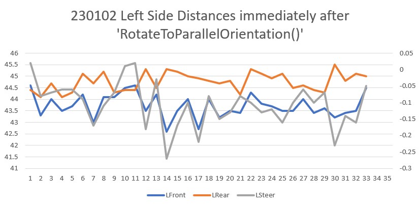
Looking at the line at time 124142, we see:
|
1 2 |
Msec LF LC LR LCCorr Steer Tweak OffCm Err LastI LastD Out Lspd Rspd 124142 29.30 31.50 29.10 31.48 0.02 -0.11 40.00 0.09 0.00 0.06 28.08 103 46 |
The steering value is very low (0.02) because the front and rear sensor distances are very close, but because the robot is well inside the intended offset distance of 40cm, the ‘tweak value’ of -0.11 is actually dominant, which drives the robot’s left motors harder than the right ones, which should correct the robot back toward 40cm offset. When we look at the Excel plot, we see:
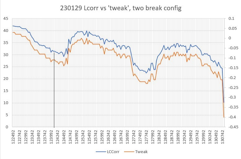
The plot shows the ‘tweak’ value becoming more negative as the corrected distance becomes smaller relative to the desired offset distance of 40cm, and thus tends to correct the robot back toward the desired offset. At the 12.41sec mark (shown by the vertical line in the above plot) the ‘tweak’ value is -0.11, compared to the steering value of +0.02, so the ‘tweak’ input should dominate the output. With a P of 300, the output with just the steering value would be -300 x 0.02 = -6 resulting in left/right motor speeds of 69/81, steering the robot very slightly toward the wall. However, with the ‘tweak’ value of -0.02 the output is -300 x (0.02 -0.11) = +27 (actually +28), resulting in motor speeds of 103/46, or moderately away from the wall, as desired.
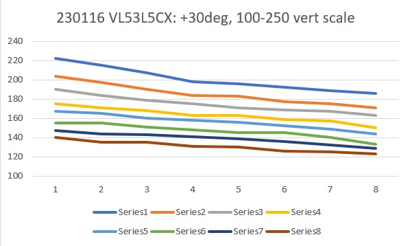
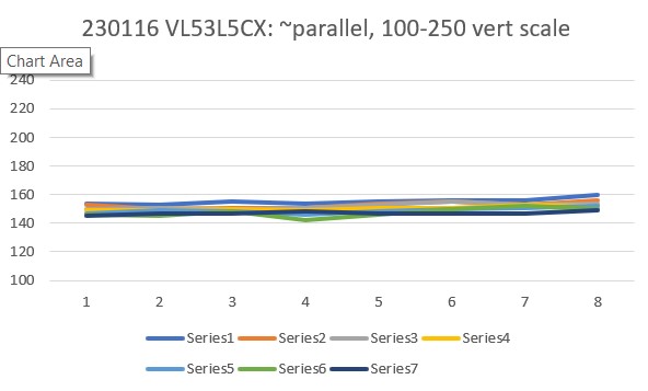
To simply the tuning problem, I changed the wall configuration back to a single straight wall, but started the robot with a 30cm offset (10cm closer than desired) but still parallel (steering value near zero). Here’s the output:
|
1 2 3 4 5 6 7 8 9 10 11 12 13 14 15 16 17 18 19 20 21 22 23 24 25 26 27 28 29 30 31 32 33 34 35 36 37 38 39 40 41 42 43 44 45 46 47 48 49 50 51 52 53 54 55 56 57 58 59 60 61 62 63 64 65 66 67 68 69 70 71 72 73 74 75 76 77 78 79 80 81 82 83 84 85 86 87 88 89 90 91 92 93 94 95 96 97 98 99 100 101 102 103 104 105 106 107 108 109 110 111 112 113 114 115 116 117 118 119 120 121 122 123 124 125 126 127 128 129 130 131 132 133 134 135 136 137 138 139 140 141 142 143 144 145 146 147 148 149 150 151 152 153 154 155 156 157 158 159 160 |
Msec LF LC LR LCCorr Steer Tweak OffCm Err LastI LastD Out Lspd Rspd 107749 29.50 32.70 28.70 32.36 0.08 -0.10 40.00 0.02 0.00 0.02 6.56 81 68 107799 30.00 32.40 28.70 31.52 0.13 -0.11 40.00 -0.02 0.00 -0.04 -5.10 69 80 107849 29.90 32.50 29.00 32.07 0.09 -0.11 40.00 0.02 0.00 0.03 4.70 79 70 107899 29.50 32.40 27.90 31.09 0.16 -0.12 40.00 -0.04 0.00 -0.06 -12.35 62 87 107949 29.40 32.00 28.50 31.58 0.09 -0.11 40.00 0.02 0.00 0.06 6.68 81 68 107999 29.50 32.70 27.80 31.21 0.17 -0.12 40.00 -0.05 0.00 -0.08 -15.84 59 90 108049 29.50 32.30 28.40 31.67 0.11 -0.11 40.00 0.00 0.00 0.05 0.32 75 74 108099 29.00 31.90 28.40 31.28 0.11 -0.12 40.00 0.01 0.00 0.01 1.88 76 73 108149 29.00 31.90 28.20 31.57 0.08 -0.11 40.00 0.03 0.00 0.03 9.72 84 65 108199 29.40 31.40 27.50 29.63 0.19 -0.14 40.00 -0.05 0.00 -0.08 -15.51 59 90 108249 28.30 31.60 27.40 31.19 0.09 -0.12 40.00 0.03 0.00 0.08 8.26 83 66 108299 28.50 31.90 27.20 31.04 0.13 -0.12 40.00 -0.01 0.00 -0.04 -3.15 71 78 108349 27.70 30.80 27.40 30.75 0.03 -0.12 40.00 0.09 0.00 0.10 27.98 102 47 108399 27.90 30.80 27.80 30.79 0.01 -0.12 40.00 0.11 0.00 0.02 33.82 108 41 108449 27.60 31.00 26.90 30.75 0.07 -0.12 40.00 0.05 0.00 -0.06 15.99 90 59 108499 28.00 30.60 26.90 30.00 0.11 -0.13 40.00 0.02 0.00 -0.03 6.98 81 68 108549 28.00 30.60 26.90 30.00 0.11 -0.13 40.00 0.02 0.00 0.00 6.98 81 68 108599 27.20 30.60 25.70 29.51 0.15 -0.14 40.00 -0.01 0.00 -0.03 -3.02 71 78 108649 26.90 30.70 25.50 29.74 0.14 -0.14 40.00 -0.00 0.00 0.01 -0.96 74 75 108699 27.20 29.90 25.50 28.54 0.17 -0.15 40.00 -0.02 0.00 -0.01 -5.15 69 80 108749 26.70 30.00 25.60 29.42 0.11 -0.14 40.00 0.03 0.00 0.05 9.34 84 65 108799 26.30 30.00 25.50 29.69 0.08 -0.14 40.00 0.06 0.00 0.03 17.24 92 57 108849 26.50 30.00 25.40 29.42 0.11 -0.14 40.00 0.03 0.00 -0.03 9.34 84 65 108899 25.60 29.30 24.80 29.00 0.08 -0.15 40.00 0.07 0.00 0.04 20.02 95 54 108949 25.60 29.10 24.70 28.72 0.09 -0.15 40.00 0.06 0.00 -0.01 18.12 93 56 108999 25.60 29.10 24.70 28.72 0.09 -0.15 40.00 0.06 0.00 0.00 18.12 93 56 109049 25.20 29.10 23.90 28.31 0.13 -0.16 40.00 0.03 0.00 -0.03 7.75 82 67 109099 25.20 29.10 23.90 28.31 0.13 -0.16 40.00 0.03 0.00 0.00 7.75 82 67 109149 25.40 28.30 24.20 27.65 0.12 -0.16 40.00 0.04 0.00 0.02 13.42 88 61 109199 25.00 27.40 24.10 27.04 0.09 -0.17 40.00 0.08 0.00 0.04 24.84 99 50 109249 24.90 27.30 24.20 27.08 0.07 -0.17 40.00 0.10 0.00 0.02 30.67 105 44 109299 24.50 28.20 23.70 27.91 0.08 -0.16 40.00 0.08 0.00 -0.02 24.37 99 50 109349 24.90 28.10 23.50 27.22 0.14 -0.17 40.00 0.03 0.00 -0.05 9.11 84 65 109399 24.20 27.80 23.50 27.58 0.07 -0.17 40.00 0.10 0.00 0.07 28.68 103 46 109449 25.00 27.40 24.10 27.04 0.09 -0.17 40.00 0.08 0.00 -0.01 24.84 99 50 109499 25.10 28.30 23.50 27.15 0.16 -0.17 40.00 0.01 0.00 -0.07 3.39 78 71 109549 25.70 28.60 24.20 27.58 0.15 -0.17 40.00 0.02 0.00 0.00 4.69 79 70 109599 25.20 30.10 24.60 29.92 0.06 -0.13 40.00 0.07 0.00 0.06 22.30 97 52 109649 25.00 28.30 24.70 28.26 0.03 -0.16 40.00 0.13 0.00 0.05 37.97 112 37 109699 25.00 28.00 24.90 28.00 0.01 -0.16 40.00 0.15 0.00 0.02 45.02 120 29 109749 25.10 28.50 24.70 28.43 0.04 -0.15 40.00 0.11 0.00 -0.04 34.30 109 40 109799 25.30 27.60 24.70 27.44 0.06 -0.17 40.00 0.11 0.00 -0.01 32.25 107 42 109849 25.60 28.30 24.70 27.93 0.09 -0.16 40.00 0.07 0.00 -0.04 21.28 96 53 109899 25.40 29.60 24.30 29.02 0.11 -0.15 40.00 0.04 0.00 -0.03 10.91 85 64 109949 26.40 824.10 24.30 767.82 0.21 9.70 40.00 -9.91 0.00 -9.95 -2974.27 0 127 109999 27.80 26.20 26.60 25.59 0.12 -0.19 40.00 0.07 0.00 9.99 21.62 96 53 110049 28.50 27.00 27.00 26.03 0.15 -0.19 40.00 0.04 0.00 -0.04 10.86 85 64 110099 28.30 27.20 26.80 26.23 0.15 -0.18 40.00 0.03 0.00 -0.00 10.09 85 64 110149 28.50 27.60 28.20 27.56 0.03 -0.17 40.00 0.14 0.00 0.10 40.76 115 34 110199 29.30 27.80 28.30 27.35 0.10 -0.17 40.00 0.07 0.00 -0.07 20.59 95 54 110249 29.50 28.90 27.80 27.58 0.17 -0.17 40.00 -0.00 0.00 -0.07 -1.33 73 76 110299 29.40 28.70 29.00 28.63 0.04 -0.15 40.00 0.11 0.00 0.12 33.50 108 41 110349 30.00 29.60 29.00 29.12 0.10 -0.15 40.00 0.05 0.00 -0.07 13.51 88 61 110399 30.80 30.00 29.20 29.19 0.13 -0.14 40.00 0.01 0.00 -0.03 4.24 79 70 110449 32.00 31.10 30.00 29.16 0.20 -0.14 40.00 -0.06 0.00 -0.07 -16.66 58 91 110499 32.60 31.00 30.30 28.49 0.23 -0.15 40.00 -0.08 0.00 -0.02 -22.94 52 97 110549 33.30 31.80 30.50 28.09 0.28 -0.16 40.00 -0.12 0.00 -0.04 -36.35 38 111 110599 32.70 32.40 31.20 31.24 0.15 -0.12 40.00 -0.03 0.00 0.09 -9.97 65 84 110649 33.70 32.90 31.90 31.23 0.18 -0.12 40.00 -0.06 0.00 -0.03 -18.91 56 93 110699 33.60 33.90 31.70 31.99 0.19 -0.11 40.00 -0.08 0.00 -0.02 -24.95 50 99 110749 33.90 33.70 32.90 33.16 0.10 -0.09 40.00 -0.01 0.00 0.07 -2.63 72 77 110799 34.40 32.90 33.00 31.87 0.14 -0.11 40.00 -0.03 0.00 -0.02 -9.49 65 84 110849 33.50 34.00 33.00 33.86 0.05 -0.08 40.00 0.03 0.00 0.06 9.55 84 65 110899 34.50 35.00 33.40 34.32 0.11 -0.08 40.00 -0.03 0.00 -0.07 -10.27 64 85 110949 34.90 34.90 33.50 33.81 0.14 -0.08 40.00 -0.06 0.00 -0.02 -17.24 57 92 110999 35.10 35.40 34.10 34.83 0.10 -0.07 40.00 -0.03 0.00 0.03 -9.32 65 84 111049 35.90 36.10 34.60 35.12 0.13 -0.07 40.00 -0.06 0.00 -0.03 -19.50 55 94 111099 36.70 35.90 34.30 34.78 0.14 -0.07 40.00 -0.07 0.00 -0.01 -21.11 53 96 111149 35.80 36.50 34.60 35.66 0.12 -0.06 40.00 -0.06 0.00 0.01 -18.63 56 93 111199 36.50 37.10 35.50 36.50 0.10 -0.05 40.00 -0.05 0.00 0.01 -16.01 58 91 111249 36.50 37.50 35.50 36.90 0.10 -0.04 40.00 -0.06 0.00 -0.01 -17.58 57 92 111299 36.20 37.60 36.10 37.59 0.01 -0.03 40.00 0.02 0.00 0.08 6.62 81 68 111349 36.40 37.60 35.80 37.38 0.06 -0.03 40.00 -0.03 0.00 -0.05 -7.52 67 82 111399 37.20 37.90 36.50 37.60 0.07 -0.03 40.00 -0.04 0.00 -0.01 -11.39 63 86 111449 37.20 37.60 36.10 36.87 0.11 -0.04 40.00 -0.07 0.00 -0.03 -20.47 54 95 111499 37.00 38.20 36.10 37.70 0.09 -0.03 40.00 -0.06 0.00 0.01 -17.80 57 92 111549 37.40 38.30 36.40 37.68 0.10 -0.03 40.00 -0.07 0.00 -0.01 -20.73 54 95 111599 38.10 38.90 36.70 37.68 0.14 -0.03 40.00 -0.11 0.00 -0.04 -32.74 42 107 111649 38.00 39.90 37.40 39.67 0.06 -0.00 40.00 -0.06 0.00 0.05 -16.67 58 91 111699 38.90 39.70 37.50 38.46 0.14 -0.02 40.00 -0.12 0.00 -0.06 -35.84 39 110 111749 39.10 39.80 38.00 39.03 0.11 -0.01 40.00 -0.10 0.00 0.02 -29.10 45 104 111799 38.40 39.50 38.00 39.40 0.04 -0.01 40.00 -0.03 0.00 0.07 -9.59 65 84 111849 38.30 40.00 37.90 39.90 0.04 -0.00 40.00 -0.04 0.00 -0.01 -11.58 63 86 111899 39.20 39.90 37.70 38.47 0.15 -0.02 40.00 -0.13 0.00 -0.09 -38.89 36 113 111949 38.40 40.00 37.90 39.84 0.05 -0.00 40.00 -0.05 0.00 0.08 -14.35 60 89 111999 38.00 39.90 37.90 39.89 0.01 -0.00 40.00 -0.01 0.00 0.04 -2.57 72 77 112049 37.30 39.40 38.40 38.63 -0.11 -0.02 40.00 0.13 0.00 0.14 38.47 113 36 112099 37.00 38.70 37.90 38.19 -0.09 -0.02 40.00 0.11 0.00 -0.01 34.23 109 40 112149 37.60 38.50 37.90 38.44 -0.03 -0.02 40.00 0.05 0.00 -0.06 15.23 90 59 112199 36.70 38.50 37.30 38.27 -0.06 -0.02 40.00 0.08 0.00 0.03 24.90 99 50 112249 36.70 37.90 36.80 37.89 -0.01 -0.03 40.00 0.04 0.00 -0.04 11.42 86 63 112299 36.90 38.10 37.10 38.08 -0.02 -0.03 40.00 0.05 0.00 0.01 13.70 88 61 112349 37.00 37.20 36.70 37.15 0.03 -0.04 40.00 0.01 0.00 -0.04 2.42 77 72 112399 36.80 37.60 36.50 37.54 0.03 -0.03 40.00 0.00 0.00 -0.01 0.82 75 74 112449 36.50 37.60 36.80 37.54 -0.03 -0.03 40.00 0.06 0.00 0.06 18.82 93 56 112499 36.10 37.70 35.60 37.55 0.05 -0.03 40.00 -0.02 0.00 -0.08 -5.19 69 80 112549 36.50 37.00 35.50 36.40 0.10 -0.05 40.00 -0.05 0.00 -0.03 -15.61 59 90 112599 36.50 37.30 36.00 37.15 0.05 -0.04 40.00 -0.01 0.00 0.04 -3.59 71 78 112649 36.80 36.50 36.50 36.45 0.03 -0.05 40.00 0.02 0.00 0.03 5.21 80 69 112699 36.00 36.80 36.30 36.75 -0.03 -0.04 40.00 0.07 0.00 0.06 22.02 97 52 112749 36.40 36.00 35.10 35.03 0.13 -0.07 40.00 -0.06 0.00 -0.14 -19.11 55 94 112799 36.00 35.90 35.10 35.43 0.09 -0.06 40.00 -0.03 0.00 0.03 -8.72 66 83 112849 34.90 36.60 35.70 36.22 -0.08 -0.05 40.00 0.13 0.00 0.16 39.12 114 35 112899 35.90 37.10 35.10 36.72 0.08 -0.04 40.00 -0.04 0.00 -0.17 -10.86 64 85 112949 35.90 36.40 35.30 36.19 0.06 -0.05 40.00 -0.01 0.00 0.03 -2.75 72 77 112999 36.30 36.10 35.00 35.12 0.13 -0.07 40.00 -0.06 0.00 -0.06 -19.50 55 94 113049 35.90 36.50 35.50 36.40 0.04 -0.05 40.00 0.01 0.00 0.07 2.38 77 72 113099 35.90 36.50 35.50 36.40 0.04 -0.05 40.00 0.01 0.00 0.00 2.38 77 72 113149 35.50 36.90 34.90 36.68 0.06 -0.04 40.00 -0.02 0.00 -0.02 -4.74 70 79 113199 35.50 36.90 34.90 36.68 0.06 -0.04 40.00 -0.02 0.00 0.00 -4.74 70 79 113249 35.80 36.90 35.70 36.89 0.01 -0.04 40.00 0.03 0.00 0.05 9.42 84 65 113299 36.00 37.20 35.20 36.81 0.08 -0.04 40.00 -0.04 0.00 -0.07 -11.26 63 86 113349 35.30 36.60 35.40 36.59 -0.01 -0.05 40.00 0.06 0.00 0.09 16.62 91 58 113399 36.70 37.30 35.70 36.70 0.10 -0.04 40.00 -0.06 0.00 -0.11 -16.79 58 91 113449 36.20 37.10 35.50 36.80 0.07 -0.04 40.00 -0.03 0.00 0.03 -8.22 66 83 113499 36.10 37.30 35.80 37.25 0.03 -0.04 40.00 0.01 0.00 0.03 2.02 77 72 113549 36.70 37.30 36.20 37.15 0.05 -0.04 40.00 -0.01 0.00 -0.02 -3.59 71 78 113599 36.60 37.20 36.20 37.10 0.04 -0.04 40.00 -0.00 0.00 0.01 -0.41 74 75 113649 36.60 37.20 36.20 37.10 0.04 -0.04 40.00 -0.00 0.00 0.00 -0.41 74 75 113699 36.90 37.90 36.20 37.60 0.07 -0.03 40.00 -0.04 0.00 -0.04 -11.39 63 86 113749 36.30 37.60 35.80 37.45 0.05 -0.03 40.00 -0.02 0.00 0.02 -4.79 70 79 113799 35.90 37.40 35.80 37.39 0.01 -0.03 40.00 0.02 0.00 0.04 7.42 82 67 113849 37.00 37.30 35.60 36.13 0.14 -0.05 40.00 -0.09 0.00 -0.11 -26.54 48 101 113899 36.60 37.50 36.10 37.35 0.05 -0.04 40.00 -0.01 0.00 0.07 -4.39 70 79 113949 36.70 38.10 35.80 37.60 0.09 -0.03 40.00 -0.06 0.00 -0.04 -17.40 57 92 113999 37.20 37.70 35.80 36.52 0.14 -0.05 40.00 -0.09 0.00 -0.04 -28.09 46 103 114049 37.00 38.10 36.80 38.08 0.02 -0.03 40.00 0.01 0.00 0.10 1.70 76 73 114099 36.70 38.40 36.30 38.30 0.04 -0.02 40.00 -0.02 0.00 -0.02 -5.20 69 80 114149 37.80 38.40 36.30 38.30 0.04 -0.02 40.00 -0.02 0.00 0.00 -5.20 69 80 114199 37.80 38.80 36.70 38.04 0.11 -0.03 40.00 -0.08 0.00 -0.07 -25.18 49 100 114249 37.00 38.00 36.50 37.85 0.05 -0.03 40.00 -0.02 0.00 0.06 -6.38 68 81 114299 37.50 38.70 36.30 37.81 0.12 -0.03 40.00 -0.09 0.00 -0.07 -27.22 47 102 114349 37.00 38.60 36.60 38.50 0.04 -0.02 40.00 -0.02 0.00 0.07 -6.00 69 80 114399 37.20 39.10 36.70 38.94 0.05 -0.01 40.00 -0.04 0.00 -0.02 -10.76 64 85 114449 37.20 38.10 36.70 37.94 0.05 -0.03 40.00 -0.02 0.00 0.01 -6.78 68 81 114499 36.70 38.10 36.60 38.09 0.01 -0.03 40.00 0.02 0.00 0.04 4.62 79 70 114549 36.50 37.10 35.80 36.80 0.07 -0.04 40.00 -0.03 0.00 -0.04 -8.22 66 83 114599 36.00 36.40 36.00 36.40 0.00 -0.05 40.00 0.05 0.00 0.08 14.40 89 60 114649 35.50 36.30 35.60 36.29 -0.01 -0.05 40.00 0.06 0.00 0.01 17.82 92 57 114699 35.90 36.40 35.50 36.31 0.04 -0.05 40.00 0.01 0.00 -0.05 2.78 77 72 114749 35.30 36.60 35.40 36.59 -0.01 -0.05 40.00 0.06 0.00 0.05 16.62 91 58 114799 34.70 35.60 34.50 35.58 0.02 -0.06 40.00 0.04 0.00 -0.02 11.69 86 63 114849 35.10 34.80 33.70 33.71 0.14 -0.08 40.00 -0.06 0.00 -0.10 -16.85 58 91 114899 34.20 35.00 33.30 34.54 0.09 -0.07 40.00 -0.02 0.00 0.04 -5.17 69 80 114949 33.70 34.20 33.40 34.15 0.03 -0.08 40.00 0.05 0.00 0.07 14.40 89 60 114999 33.70 34.20 33.40 34.15 0.03 -0.08 40.00 0.05 0.00 0.00 14.40 89 60 115049 33.00 33.20 32.60 33.11 0.04 -0.09 40.00 0.05 0.00 0.00 15.55 90 59 115099 33.00 33.20 32.60 33.11 0.04 -0.09 40.00 0.05 0.00 0.00 15.55 90 59 115149 32.60 32.30 32.10 32.17 0.05 -0.10 40.00 0.05 0.00 0.00 16.33 91 58 115199 31.80 31.30 30.90 30.89 0.09 -0.12 40.00 0.03 0.00 -0.02 9.44 84 65 115249 30.90 31.00 30.30 30.82 0.06 -0.12 40.00 0.06 0.00 0.03 18.73 93 56 115299 31.00 30.50 29.90 29.91 0.11 -0.13 40.00 0.02 0.00 -0.04 7.38 82 67 115349 31.00 29.70 29.80 29.01 0.12 -0.15 40.00 0.03 0.00 0.00 7.94 82 67 115399 30.50 29.90 29.10 28.97 0.14 -0.15 40.00 0.01 0.00 -0.02 2.14 77 72 115449 29.30 29.20 28.10 28.53 0.12 -0.15 40.00 0.03 0.00 0.03 9.90 84 65 115499 29.60 28.90 27.80 27.43 0.18 -0.17 40.00 -0.01 0.00 -0.05 -3.72 71 78 115549 29.60 28.90 27.80 27.43 0.18 -0.17 40.00 -0.01 0.00 0.00 -3.72 71 78 115599 29.90 28.30 27.90 26.54 0.20 -0.18 40.00 -0.02 0.00 -0.01 -6.15 68 81 115649 31.50 824.10 28.50 715.07 0.30 9.00 40.00 -9.30 0.00 -9.28 -2790.27 0 127 |
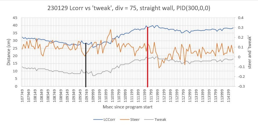
As can be seen from the above plot, the robot starts out at about 32cm, and slowly closes to about 28cm. Simultaneously the ‘tweak’ value goes from about -0.12 to about -0.18 (at 109749 mSec, the black line). The result is the robot starts moving away from the wall, getting to the desired 40cm offset a little over 2sec later (the red line). After this point it maintains about 40cm offset, as desired. The average offset distance from the red line to the end of the run is about 37.5cm – nice!
So it looks like P = 300 and tweak divisor = 75 is a nice starting point.
30 January 2023 Update:
Now that I have both the PID and divisor values as parameters, I plan to make some more ‘straight wall’ runs to see how the robot behaves. My belief is that a slightly lower divisor ratio, and possibly a slightly higher P value will be beneficial – we’ll see
Starting with P = 300 and divisor = 50:
|
1 2 3 4 5 6 7 8 9 10 11 12 13 14 15 16 17 18 19 20 21 22 23 24 25 26 27 28 29 30 31 32 33 34 35 36 37 38 39 40 41 42 43 44 45 46 47 48 49 50 51 52 53 54 55 56 57 58 59 60 61 62 63 64 65 66 67 68 69 70 71 72 73 74 75 76 77 78 79 80 81 82 83 84 85 86 87 88 89 90 91 92 93 94 95 96 97 98 99 100 101 102 103 104 105 106 107 108 109 110 111 112 113 114 115 116 117 118 119 120 121 122 123 124 125 126 127 128 129 130 131 132 133 134 135 136 137 138 139 140 141 142 143 144 145 146 147 148 |
Front Center Rear Steer 33.10 33.40 31.40 0.17 WallE3_WallTrackTuning_V5.ino: TrackLeftWallOffset: Start tracking offset of 40.0 cm with Kp/Ki/Kd = 300.00 0.00 0.00 Msec LF LC LR Steer Deg Cos LCCorr Set Err SpinDeg WallE3_WallTrackTuning_V5.ino: In TrackLeftWallOffset: before while with errcode = NO_ANOMALIES Msec LF LC LR LCCorr Steer Tweak OffCm Err LastI LastD Out Lspd Rspd 1065957 32.50 33.40 31.60 33.13 0.07 -0.14 40.00 0.07 0.00 0.07 20.19 95 54 1066007 32.50 33.40 31.20 32.50 0.13 -0.15 40.00 0.02 0.00 -0.05 6.02 81 68 1066057 32.60 33.20 31.10 32.01 0.15 -0.16 40.00 0.01 0.00 -0.01 2.92 77 72 1066107 33.20 33.70 31.10 31.40 0.21 -0.17 40.00 -0.04 0.00 -0.05 -11.39 63 86 1066157 32.70 34.10 31.70 33.55 0.10 -0.13 40.00 0.03 0.00 0.07 8.70 83 66 1066207 33.50 34.90 32.10 33.81 0.14 -0.12 40.00 -0.02 0.00 -0.05 -4.86 70 79 1066257 33.60 33.60 32.20 32.55 0.14 -0.15 40.00 0.01 0.00 0.03 2.70 77 72 1066307 34.10 34.80 32.70 33.71 0.14 -0.13 40.00 -0.01 0.00 -0.02 -4.28 70 79 1066357 33.90 35.50 33.30 35.29 0.06 -0.09 40.00 0.03 0.00 0.05 10.25 85 64 1066407 33.90 35.50 33.30 35.29 0.06 -0.09 40.00 0.03 0.00 0.00 10.25 85 64 1066457 34.70 35.90 33.20 34.62 0.15 -0.11 40.00 -0.04 0.00 -0.08 -12.70 62 87 1066507 34.70 35.80 33.90 35.43 0.08 -0.09 40.00 0.01 0.00 0.05 3.43 78 71 1066557 34.90 36.20 34.00 35.73 0.09 -0.09 40.00 -0.00 0.00 -0.02 -1.36 73 76 1066607 35.10 36.80 33.90 35.95 0.12 -0.08 40.00 -0.04 0.00 -0.03 -11.70 63 86 1066657 36.10 36.80 34.80 35.81 0.13 -0.08 40.00 -0.05 0.00 -0.01 -13.83 61 88 1066707 35.60 37.00 34.60 36.40 0.10 -0.07 40.00 -0.03 0.00 0.02 -8.42 66 83 1066757 35.60 37.40 35.00 37.18 0.06 -0.06 40.00 -0.00 0.00 0.02 -1.09 73 76 1066807 36.00 37.30 34.80 36.44 0.12 -0.07 40.00 -0.05 0.00 -0.05 -14.63 60 89 1066857 35.50 36.80 35.10 36.70 0.04 -0.07 40.00 0.03 0.00 0.07 7.78 82 67 1066907 35.90 37.60 35.60 37.54 0.03 -0.05 40.00 0.02 0.00 -0.01 5.73 80 69 1066957 36.80 37.60 35.10 35.89 0.17 -0.08 40.00 -0.09 0.00 -0.11 -26.32 48 101 1067007 36.40 38.00 35.30 37.26 0.11 -0.05 40.00 -0.06 0.00 0.03 -16.56 58 91 1067057 36.50 38.10 35.10 36.91 0.14 -0.06 40.00 -0.08 0.00 -0.02 -23.46 51 98 1067107 37.00 38.20 35.60 37.90 0.07 -0.04 40.00 -0.03 0.00 0.05 -8.38 66 83 1067157 37.40 37.90 36.60 37.51 0.08 -0.05 40.00 -0.03 0.00 -0.00 -9.04 65 84 1067207 36.90 38.20 36.10 37.80 0.08 -0.04 40.00 -0.04 0.00 -0.01 -10.82 64 85 1067257 37.40 38.50 36.30 37.75 0.11 -0.04 40.00 -0.07 0.00 -0.03 -19.50 55 94 1067307 36.40 38.50 36.00 38.40 0.04 -0.03 40.00 -0.01 0.00 0.06 -2.40 72 77 1067357 36.50 38.20 36.50 38.20 0.00 -0.04 40.00 0.04 0.00 0.04 10.80 85 64 1067407 36.80 38.10 36.90 38.09 -0.01 -0.04 40.00 0.05 0.00 0.01 14.44 89 60 1067457 36.50 38.50 36.40 38.49 0.01 -0.03 40.00 0.02 0.00 -0.03 6.04 81 68 1067507 37.00 38.40 35.70 37.36 0.13 -0.05 40.00 -0.08 0.00 -0.10 -23.17 51 98 1067557 37.40 38.70 37.10 38.64 0.03 -0.03 40.00 -0.00 0.00 0.07 -0.86 74 75 1067607 37.60 38.50 36.20 37.30 0.14 -0.05 40.00 -0.09 0.00 -0.08 -25.78 49 100 1067657 37.00 38.60 36.60 38.50 0.04 -0.03 40.00 -0.01 0.00 0.08 -3.00 72 77 1067707 37.30 38.60 36.40 38.09 0.09 -0.04 40.00 -0.05 0.00 -0.04 -15.57 59 90 1067757 37.40 38.30 36.50 37.80 0.09 -0.04 40.00 -0.05 0.00 0.01 -13.79 61 88 1067807 37.90 39.50 36.50 38.27 0.14 -0.03 40.00 -0.11 0.00 -0.06 -31.59 43 106 1067857 36.80 38.30 36.60 38.27 0.02 -0.03 40.00 0.01 0.00 0.12 4.35 79 70 1067907 37.20 38.80 36.70 38.64 0.05 -0.03 40.00 -0.02 0.00 -0.04 -6.85 68 81 1067957 37.20 38.70 36.90 38.64 0.03 -0.03 40.00 -0.00 0.00 0.02 -0.86 74 75 1068007 37.10 37.60 36.70 37.50 0.04 -0.05 40.00 0.01 0.00 0.01 2.99 77 72 1068057 36.70 38.70 36.50 38.67 0.02 -0.03 40.00 0.01 0.00 -0.00 1.95 76 73 1068107 35.70 37.90 36.20 37.75 -0.05 -0.05 40.00 0.10 0.00 0.09 28.53 103 46 1068157 35.30 37.30 35.90 37.08 -0.06 -0.06 40.00 0.12 0.00 0.02 35.51 110 39 1068207 35.20 37.30 35.60 37.20 -0.04 -0.06 40.00 0.10 0.00 -0.02 28.78 103 46 1068257 35.20 36.50 34.70 36.35 0.05 -0.07 40.00 0.02 0.00 -0.07 6.89 81 68 1068307 34.90 36.60 35.20 36.55 -0.03 -0.07 40.00 0.10 0.00 0.08 29.72 104 45 1068357 35.10 36.20 34.50 36.05 0.05 -0.08 40.00 0.03 0.00 -0.07 8.68 83 66 1068407 34.60 36.10 34.70 36.09 -0.01 -0.08 40.00 0.09 0.00 0.06 26.44 101 48 1068457 33.70 36.40 34.20 36.25 -0.05 -0.07 40.00 0.12 0.00 0.04 37.49 112 37 1068507 34.40 36.40 34.10 36.35 0.03 -0.07 40.00 0.04 0.00 -0.08 12.92 87 62 1068557 34.70 36.00 34.20 35.79 0.06 -0.08 40.00 0.02 0.00 -0.02 7.26 82 67 1068607 33.90 36.00 33.40 35.85 0.05 -0.08 40.00 0.03 0.00 0.01 9.88 84 65 1068657 34.60 35.60 34.10 35.46 0.05 -0.09 40.00 0.04 0.00 0.01 12.27 87 62 1068707 34.80 35.30 33.80 34.73 0.10 -0.11 40.00 0.01 0.00 -0.04 1.62 76 73 1068757 35.10 36.00 34.00 35.30 0.11 -0.09 40.00 -0.02 0.00 -0.02 -4.79 70 79 1068807 33.90 35.90 34.60 35.61 -0.07 -0.09 40.00 0.16 0.00 0.17 47.31 122 27 1068857 34.30 36.10 33.90 36.01 0.04 -0.08 40.00 0.04 0.00 -0.12 11.96 86 63 1068907 34.60 36.50 33.70 36.02 0.09 -0.08 40.00 -0.01 0.00 -0.05 -3.13 71 78 1068957 35.10 36.80 33.90 35.95 0.12 -0.08 40.00 -0.04 0.00 -0.03 -11.70 63 86 1069007 35.20 35.90 35.10 35.89 0.01 -0.08 40.00 0.07 0.00 0.11 21.64 96 53 1069057 35.50 37.10 34.90 36.88 0.06 -0.06 40.00 0.00 0.00 -0.07 0.70 75 74 1069107 35.70 36.40 34.90 36.02 0.08 -0.08 40.00 -0.00 0.00 -0.00 -0.14 74 75 1069157 35.20 37.10 34.30 36.61 0.09 -0.07 40.00 -0.02 0.00 -0.02 -6.68 68 81 1069207 35.80 37.30 35.00 37.30 0.00 -0.05 40.00 0.05 0.00 0.08 16.20 91 58 1069257 36.90 36.60 35.70 35.75 0.12 -0.08 40.00 -0.04 0.00 -0.09 -10.53 64 85 1069307 36.70 37.70 35.80 37.21 0.09 -0.06 40.00 -0.03 0.00 0.00 -10.24 64 85 1069357 35.90 37.70 35.30 37.48 0.06 -0.05 40.00 -0.01 0.00 0.02 -2.88 72 77 1069407 36.10 37.00 35.30 36.62 0.08 -0.07 40.00 -0.01 0.00 -0.00 -3.70 71 78 1069457 35.90 38.10 35.20 37.80 0.07 -0.04 40.00 -0.03 0.00 -0.01 -7.78 67 82 1069507 36.60 37.50 36.20 37.40 0.04 -0.05 40.00 0.01 0.00 0.04 3.59 78 71 1069557 35.80 39.20 35.90 39.19 -0.01 -0.02 40.00 0.03 0.00 0.01 7.84 82 67 1069607 36.30 38.70 35.40 38.19 0.09 -0.04 40.00 -0.05 0.00 -0.08 -16.16 58 91 1069657 36.10 38.00 36.50 37.90 -0.04 -0.04 40.00 0.08 0.00 0.14 24.59 99 50 1069707 37.00 38.70 36.50 38.54 0.05 -0.03 40.00 -0.02 0.00 -0.10 -6.25 68 81 1069757 37.30 38.80 35.20 36.15 0.21 -0.08 40.00 -0.13 0.00 -0.11 -39.90 35 114 1069807 37.00 39.20 36.30 38.89 0.07 -0.02 40.00 -0.05 0.00 0.09 -14.33 60 89 1069857 37.90 39.00 36.20 37.22 0.17 -0.06 40.00 -0.11 0.00 -0.07 -34.34 40 109 1069907 38.10 39.70 36.70 38.46 0.14 -0.03 40.00 -0.11 0.00 0.01 -32.76 42 107 1069957 37.00 39.10 37.20 39.07 -0.02 -0.02 40.00 0.04 0.00 0.15 11.55 86 63 1070007 37.00 40.10 37.20 40.07 -0.02 0.00 40.00 0.02 0.00 -0.02 5.56 80 69 1070057 36.80 39.40 37.00 39.37 -0.02 -0.01 40.00 0.03 0.00 0.01 9.75 84 65 1070107 37.30 39.10 37.10 39.07 0.02 -0.02 40.00 -0.00 0.00 -0.03 -0.45 74 75 1070157 37.20 39.70 37.10 39.69 0.01 -0.01 40.00 -0.00 0.00 -0.00 -1.16 73 76 1070207 37.10 39.10 37.10 39.10 0.00 -0.02 40.00 0.02 0.00 0.02 5.40 80 69 1070257 37.40 38.50 37.60 38.47 -0.02 -0.03 40.00 0.05 0.00 0.03 15.15 90 59 1070307 37.00 39.00 37.10 38.99 -0.01 -0.02 40.00 0.03 0.00 -0.02 9.04 84 65 1070357 36.40 38.70 37.00 38.70 0.00 -0.03 40.00 0.03 0.00 -0.00 7.80 82 67 1070407 35.60 38.50 36.50 38.00 -0.09 -0.04 40.00 0.13 0.00 0.10 39.03 114 35 1070457 37.00 38.10 36.30 37.80 0.07 -0.04 40.00 -0.03 0.00 -0.16 -7.78 67 82 1070507 36.10 38.40 36.40 38.34 -0.03 -0.03 40.00 0.06 0.00 0.09 18.94 93 56 1070557 35.80 36.90 35.50 36.85 0.03 -0.06 40.00 0.03 0.00 -0.03 9.93 84 65 1070607 35.10 38.00 35.70 37.78 -0.06 -0.04 40.00 0.10 0.00 0.07 31.33 106 43 1070657 35.20 37.10 35.40 37.08 -0.02 -0.06 40.00 0.08 0.00 -0.03 23.55 98 51 1070707 35.20 37.60 35.20 37.60 0.00 -0.05 40.00 0.05 0.00 -0.03 14.40 89 60 1070757 35.20 36.90 34.90 36.85 0.03 -0.06 40.00 0.03 0.00 -0.01 9.93 84 65 1070807 36.00 37.30 34.80 36.44 0.12 -0.07 40.00 -0.05 0.00 -0.08 -14.63 60 89 1070857 35.10 37.20 34.90 37.18 0.02 -0.06 40.00 0.04 0.00 0.09 10.95 85 64 1070907 35.40 37.10 34.70 36.80 0.07 -0.06 40.00 -0.01 0.00 -0.04 -1.83 73 76 1070957 35.80 37.00 35.00 36.62 0.08 -0.07 40.00 -0.01 0.00 -0.01 -3.70 71 78 1071007 35.20 37.80 34.70 37.65 0.05 -0.05 40.00 -0.00 0.00 0.01 -0.88 74 75 1071057 35.30 37.50 35.10 37.48 0.02 -0.05 40.00 0.03 0.00 0.03 9.15 84 65 1071107 35.90 36.90 34.40 35.58 0.15 -0.09 40.00 -0.06 0.00 -0.09 -18.49 56 93 1071157 35.90 37.30 35.40 37.15 0.05 -0.06 40.00 0.01 0.00 0.07 2.11 77 72 1071207 35.60 37.20 34.80 36.81 0.08 -0.06 40.00 -0.02 0.00 -0.02 -4.89 70 79 1071257 36.20 37.10 35.40 37.08 -0.02 -0.06 40.00 0.08 0.00 0.09 23.55 98 51 1071307 36.00 37.20 35.50 37.15 0.03 -0.06 40.00 0.03 0.00 -0.05 8.13 83 66 1071357 35.90 37.70 33.80 35.13 0.21 -0.10 40.00 -0.11 0.00 -0.14 -33.75 41 108 1071407 36.00 38.40 35.40 38.18 0.06 -0.04 40.00 -0.02 0.00 0.09 -7.05 67 82 1071457 35.80 38.20 35.30 38.04 0.05 -0.04 40.00 -0.01 0.00 0.01 -3.27 71 78 1071507 35.70 37.50 35.80 37.49 -0.01 -0.05 40.00 0.06 0.00 0.07 18.04 93 56 1071557 35.50 37.30 35.50 37.30 0.00 -0.05 40.00 0.05 0.00 -0.01 16.20 91 58 1071607 35.90 38.40 35.30 38.18 0.06 -0.04 40.00 -0.02 0.00 -0.08 -7.05 67 82 1071657 36.10 38.30 35.40 38.00 0.07 -0.04 40.00 -0.03 0.00 -0.01 -8.97 66 83 1071707 35.90 37.80 36.00 37.79 -0.01 -0.04 40.00 0.05 0.00 0.08 16.24 91 58 1071757 36.20 38.80 36.30 38.79 -0.01 -0.02 40.00 0.03 0.00 -0.02 10.24 85 64 1071807 37.00 38.90 35.70 37.85 0.13 -0.04 40.00 -0.09 0.00 -0.12 -26.09 48 101 1071857 37.00 38.70 35.80 37.81 0.12 -0.04 40.00 -0.08 0.00 0.01 -22.84 52 97 1071907 36.90 38.90 36.30 38.67 0.06 -0.03 40.00 -0.03 0.00 0.04 -10.03 64 85 1071957 37.50 39.40 37.10 39.17 -0.06 -0.02 40.00 0.08 0.00 0.11 22.98 97 52 1072007 37.40 40.50 35.30 37.73 0.21 -0.05 40.00 -0.16 0.00 -0.24 -49.40 25 124 1072057 38.10 39.70 36.80 38.63 0.13 -0.03 40.00 -0.10 0.00 0.06 -30.76 44 105 1072107 37.80 39.20 37.70 39.19 0.01 -0.02 40.00 0.01 0.00 0.11 1.84 76 73 1072157 38.50 39.80 36.70 37.78 0.18 -0.04 40.00 -0.14 0.00 -0.14 -40.65 34 115 1072207 37.90 40.60 38.00 40.59 -0.01 0.01 40.00 -0.00 0.00 0.13 -0.56 74 75 1072257 38.60 39.40 37.60 38.76 0.10 -0.02 40.00 -0.08 0.00 -0.07 -22.59 52 97 1072307 38.60 40.20 38.00 39.96 0.06 -0.00 40.00 -0.06 0.00 0.02 -17.79 57 92 1072357 38.60 40.60 38.10 40.43 0.05 0.01 40.00 -0.06 0.00 0.00 -17.61 57 92 1072407 38.70 40.50 36.90 38.44 0.18 -0.03 40.00 -0.15 0.00 -0.09 -44.64 30 119 1072457 38.30 41.20 36.80 39.73 0.15 -0.01 40.00 -0.14 0.00 0.00 -43.36 31 118 1072507 37.80 40.40 37.50 40.34 0.03 0.01 40.00 -0.04 0.00 0.11 -11.04 63 86 1072557 38.20 40.80 37.30 40.27 0.09 0.01 40.00 -0.10 0.00 -0.06 -28.59 46 103 1072607 37.80 40.30 38.00 40.27 -0.02 0.01 40.00 0.01 0.00 0.11 4.36 79 70 1072657 38.00 39.40 37.90 39.39 0.01 -0.01 40.00 0.00 0.00 -0.01 0.64 75 74 1072707 37.10 39.00 38.30 38.10 -0.12 -0.04 40.00 0.16 0.00 0.16 47.41 122 27 1072757 37.30 39.60 37.50 39.57 -0.02 -0.01 40.00 0.03 0.00 -0.13 8.56 83 66 1072807 36.40 37.90 38.80 34.57 -0.24 -0.11 40.00 0.35 0.00 0.32 104.57 127 0 1072857 36.40 38.30 36.90 38.14 -0.05 -0.04 40.00 0.09 0.00 -0.26 26.14 101 48 1072907 35.10 36.10 37.20 33.63 -0.21 -0.13 40.00 0.34 0.00 0.25 101.19 127 0 |
This run started with the robot placed roughly parallel to and offset about 32cm from the start of the 4m straight wall section. For the first two seconds the offset increased monotonically to about 38cm, and after that the robot maintained an offset between 35 and 39cm. The average for the ‘maintenance’ portion of the run was approximately 38cm – nice!
PID(350,0,0), divisor = 50:
|
1 2 3 4 5 6 7 8 9 10 11 12 13 14 15 16 17 18 19 20 21 22 23 24 25 26 27 28 29 30 31 32 33 34 35 36 37 38 39 40 41 42 43 44 45 46 47 48 49 50 51 52 53 54 55 56 57 58 59 60 61 62 63 64 65 66 67 68 69 70 71 72 73 74 75 76 77 78 79 80 81 82 83 84 85 86 87 88 89 90 91 92 93 94 95 96 97 98 99 100 101 102 103 104 105 106 107 108 109 110 111 112 113 114 115 116 117 118 119 120 121 122 123 124 125 126 127 128 129 130 131 132 133 134 135 136 137 138 139 140 141 142 143 144 145 146 147 148 149 150 151 152 153 154 155 156 157 158 159 160 161 162 163 164 165 166 167 |
Front Center Rear Steer 26.90 29.20 26.30 0.06 26.60 28.60 25.80 0.12 26.90 28.30 25.80 0.11 WallE3_WallTrackTuning_V5.ino: TrackLeftWallOffset: Start tracking offset of 40.0 cm with Kp/Ki/Kd = 350.00 0.00 0.00 Msec LF LC LR Steer Deg Cos LCCorr Set Err SpinDeg WallE3_WallTrackTuning_V5.ino: In TrackLeftWallOffset: before while with errcode = NO_ANOMALIES Msec LF LC LR LCCorr Steer Tweak OffCm Err LastI LastD Out Lspd Rspd 83213 27.70 27.60 26.30 26.74 0.14 -0.27 40.00 0.13 0.00 0.13 43.84 118 31 83263 27.70 27.40 27.20 27.29 0.05 -0.25 40.00 0.20 0.00 0.08 71.48 127 3 83313 27.80 27.50 26.70 26.96 0.11 -0.26 40.00 0.15 0.00 -0.05 52.75 127 22 83363 28.20 27.00 26.30 25.48 0.19 -0.29 40.00 0.10 0.00 -0.05 35.17 110 39 83413 28.20 27.80 26.30 26.23 0.19 -0.28 40.00 0.09 0.00 -0.02 29.88 104 45 83463 28.90 28.10 26.40 25.44 0.25 -0.29 40.00 0.04 0.00 -0.04 14.44 89 60 83513 29.80 29.60 27.10 26.37 0.27 -0.27 40.00 0.00 0.00 -0.04 0.93 75 74 83563 30.00 30.40 28.30 29.01 0.17 -0.22 40.00 0.05 0.00 0.05 17.40 92 57 83613 31.00 31.50 29.00 29.54 0.20 -0.21 40.00 0.01 0.00 -0.04 3.22 78 71 83663 31.90 31.30 30.10 29.71 0.18 -0.21 40.00 0.03 0.00 0.02 9.05 84 65 83713 32.70 31.40 29.40 26.48 0.33 -0.27 40.00 -0.06 0.00 -0.09 -20.83 54 95 83763 32.70 33.90 30.80 31.99 0.19 -0.16 40.00 -0.03 0.00 0.03 -10.41 64 85 83813 33.90 34.80 30.70 29.63 0.32 -0.21 40.00 -0.11 0.00 -0.08 -39.42 35 114 83863 34.50 35.20 31.70 31.09 0.28 -0.18 40.00 -0.10 0.00 0.01 -35.63 39 110 83913 34.40 35.40 32.50 33.40 0.19 -0.13 40.00 -0.06 0.00 0.04 -20.32 54 95 83963 35.20 35.70 33.30 33.69 0.19 -0.13 40.00 -0.06 0.00 -0.01 -22.30 52 97 84013 35.60 36.60 33.20 33.39 0.24 -0.13 40.00 -0.11 0.00 -0.04 -37.70 37 112 84063 35.90 36.70 33.70 33.96 0.22 -0.12 40.00 -0.10 0.00 0.01 -34.74 40 109 84113 36.50 37.50 34.60 36.77 0.11 -0.06 40.00 -0.05 0.00 0.05 -15.89 59 90 84163 37.00 38.40 34.40 34.49 0.26 -0.11 40.00 -0.15 0.00 -0.10 -52.41 22 127 84213 36.50 38.00 35.30 37.12 0.12 -0.06 40.00 -0.06 0.00 0.09 -21.85 53 96 84263 36.30 37.90 35.40 37.40 0.09 -0.05 40.00 -0.04 0.00 0.02 -13.33 61 88 84313 36.80 37.30 35.40 36.13 0.14 -0.08 40.00 -0.06 0.00 -0.02 -21.94 53 96 84363 36.60 37.70 35.50 36.97 0.11 -0.06 40.00 -0.05 0.00 0.01 -17.26 57 92 84413 36.50 37.90 35.80 37.60 0.07 -0.05 40.00 -0.02 0.00 0.03 -7.69 67 82 84463 36.30 38.50 35.40 38.00 0.09 -0.04 40.00 -0.05 0.00 -0.03 -17.47 57 92 84513 36.70 38.20 36.20 38.04 0.05 -0.04 40.00 -0.01 0.00 0.04 -3.81 71 78 84563 37.10 37.80 35.90 36.93 0.12 -0.06 40.00 -0.06 0.00 -0.05 -20.49 54 95 84613 36.50 38.20 35.80 37.90 0.07 -0.04 40.00 -0.03 0.00 0.03 -9.77 65 84 84663 37.50 38.00 36.00 36.64 0.15 -0.07 40.00 -0.08 0.00 -0.05 -28.99 46 103 84713 37.00 37.60 35.70 36.58 0.13 -0.07 40.00 -0.06 0.00 0.02 -21.59 53 96 84763 37.00 37.50 36.80 37.48 0.02 -0.05 40.00 0.03 0.00 0.09 10.67 85 64 84813 36.70 37.00 36.30 36.90 0.04 -0.06 40.00 0.02 0.00 -0.01 7.68 82 67 84863 36.40 37.80 36.00 37.70 0.04 -0.05 40.00 0.01 0.00 -0.02 2.09 77 72 84913 36.90 38.20 35.80 37.46 0.11 -0.05 40.00 -0.06 0.00 -0.07 -20.69 54 95 84963 36.20 38.40 36.30 38.39 -0.01 -0.03 40.00 0.04 0.00 0.10 14.74 89 60 85013 36.30 37.40 35.40 36.91 0.09 -0.06 40.00 -0.03 0.00 -0.07 -9.87 65 84 85063 35.90 37.60 35.10 37.21 0.08 -0.06 40.00 -0.02 0.00 0.00 -8.47 66 83 85113 35.40 37.30 35.50 37.29 -0.01 -0.05 40.00 0.06 0.00 0.09 22.44 97 52 85163 36.00 37.00 35.10 36.52 0.09 -0.07 40.00 -0.02 0.00 -0.08 -7.11 67 82 85213 36.10 38.10 35.10 37.49 0.10 -0.05 40.00 -0.05 0.00 -0.03 -17.40 57 92 85263 35.20 37.10 35.60 37.00 -0.04 -0.06 40.00 0.10 0.00 0.15 34.98 109 40 85313 36.10 37.10 35.80 37.05 0.03 -0.06 40.00 0.03 0.00 -0.07 10.18 85 64 85363 35.20 36.50 34.80 36.40 0.04 -0.07 40.00 0.03 0.00 0.00 11.17 86 63 85413 34.70 35.70 34.70 35.70 0.00 -0.09 40.00 0.09 0.00 0.05 30.10 105 44 85463 34.30 36.30 34.60 36.25 -0.03 -0.08 40.00 0.11 0.00 0.02 36.77 111 38 85513 34.70 35.60 34.40 35.55 0.03 -0.09 40.00 0.06 0.00 -0.05 20.67 95 54 85563 34.40 35.20 33.80 34.99 0.06 -0.10 40.00 0.04 0.00 -0.02 14.04 89 60 85613 34.10 34.70 33.90 34.68 0.02 -0.11 40.00 0.09 0.00 0.05 30.26 105 44 85663 34.20 34.90 34.10 34.89 0.01 -0.10 40.00 0.09 0.00 0.01 32.24 107 42 85713 33.90 34.90 33.40 34.76 0.05 -0.10 40.00 0.05 0.00 -0.04 19.19 94 55 85763 33.50 35.00 33.50 35.00 0.00 -0.10 40.00 0.10 0.00 0.05 35.00 110 40 85813 34.20 34.80 33.60 34.60 0.06 -0.11 40.00 0.05 0.00 -0.05 16.83 91 58 85863 34.00 35.30 32.50 34.04 0.15 -0.12 40.00 -0.03 0.00 -0.08 -10.77 64 85 85913 34.10 34.80 33.40 34.52 0.07 -0.11 40.00 0.04 0.00 0.07 13.84 88 61 85963 33.70 35.40 33.50 35.38 0.02 -0.09 40.00 0.07 0.00 0.03 25.36 100 49 86013 35.30 36.00 33.00 33.08 0.23 -0.14 40.00 -0.09 0.00 -0.16 -32.07 42 107 86063 34.40 34.90 33.60 34.54 0.08 -0.11 40.00 0.03 0.00 0.12 10.23 85 64 86113 34.80 35.50 33.60 34.68 0.12 -0.11 40.00 -0.01 0.00 -0.04 -4.76 70 79 86163 35.20 35.60 34.20 35.39 0.06 -0.09 40.00 0.03 0.00 0.05 11.26 86 63 86213 34.80 36.00 34.00 35.63 0.08 -0.09 40.00 0.01 0.00 -0.02 2.61 77 72 86263 34.10 36.30 34.00 36.29 0.01 -0.07 40.00 0.06 0.00 0.06 22.44 97 52 86313 35.00 35.90 34.60 35.81 0.04 -0.08 40.00 0.04 0.00 -0.02 15.36 90 59 86363 36.10 36.20 34.10 33.95 0.20 -0.12 40.00 -0.08 0.00 -0.12 -27.63 47 102 86413 35.50 36.70 35.60 36.69 -0.01 -0.07 40.00 0.08 0.00 0.16 26.64 101 48 86463 36.70 36.90 35.20 35.58 0.15 -0.09 40.00 -0.06 0.00 -0.14 -21.57 53 96 86513 36.10 37.30 34.90 36.44 0.12 -0.07 40.00 -0.05 0.00 0.01 -17.07 57 92 86563 36.90 37.60 35.20 35.89 0.17 -0.08 40.00 -0.09 0.00 -0.04 -30.71 44 105 86613 36.20 37.70 35.80 37.60 0.04 -0.05 40.00 0.01 0.00 0.10 2.79 77 72 86663 36.40 37.50 35.80 37.48 0.02 -0.05 40.00 0.03 0.00 0.02 10.67 85 64 86713 36.90 37.80 36.50 37.79 -0.01 -0.04 40.00 0.05 0.00 0.02 18.94 93 56 86763 36.50 38.20 36.00 38.04 0.05 -0.04 40.00 -0.01 0.00 -0.07 -3.81 71 78 86813 36.80 38.60 36.70 38.59 0.01 -0.03 40.00 0.02 0.00 0.03 6.34 81 68 86863 37.00 39.60 36.80 39.57 0.02 -0.01 40.00 -0.01 0.00 -0.03 -4.02 70 79 86913 37.00 39.30 37.00 39.30 0.00 -0.01 40.00 0.01 0.00 0.03 4.90 79 70 86963 38.00 38.70 37.40 38.47 0.06 -0.03 40.00 -0.03 0.00 -0.04 -10.31 64 85 87013 38.00 39.20 37.10 38.69 0.09 -0.03 40.00 -0.06 0.00 -0.03 -22.31 52 97 87063 38.00 40.10 37.70 40.09 -0.01 0.00 40.00 0.01 0.00 0.07 2.85 77 72 87113 38.30 40.40 37.20 39.47 0.12 -0.01 40.00 -0.11 0.00 -0.12 -38.27 36 113 87163 38.10 40.00 37.10 39.35 0.10 -0.01 40.00 -0.09 0.00 0.02 -30.48 44 105 87213 38.20 40.50 38.50 40.44 -0.03 0.01 40.00 0.02 0.00 0.11 7.42 82 67 87263 39.00 40.70 37.70 39.60 0.13 -0.01 40.00 -0.12 0.00 -0.14 -42.70 32 117 87313 39.70 40.40 37.90 38.34 0.18 -0.03 40.00 -0.15 0.00 -0.02 -51.41 23 126 87363 38.50 40.40 38.60 40.24 -0.05 0.00 40.00 0.05 0.00 0.19 15.85 90 59 87413 38.20 41.40 39.30 41.34 -0.03 0.03 40.00 0.00 0.00 -0.04 1.13 76 73 87463 39.30 40.00 38.40 39.48 0.09 -0.01 40.00 -0.08 0.00 -0.08 -27.83 47 102 87513 39.30 40.60 38.40 40.07 0.09 0.00 40.00 -0.09 0.00 -0.01 -31.98 43 106 87563 38.50 40.10 38.90 40.00 -0.04 -0.00 40.00 0.04 0.00 0.13 14.03 89 60 87613 38.00 40.30 38.30 40.24 -0.03 0.00 40.00 0.03 0.00 -0.01 8.81 83 66 87663 38.50 40.50 38.60 40.49 -0.01 0.01 40.00 0.00 0.00 -0.03 0.05 75 74 87713 36.90 39.30 37.70 38.89 -0.08 -0.02 40.00 0.10 0.00 0.10 35.75 110 39 87763 38.10 38.60 38.30 38.57 -0.02 -0.03 40.00 0.05 0.00 -0.05 16.98 91 58 87813 37.40 38.80 37.50 38.79 -0.01 -0.02 40.00 0.03 0.00 -0.01 11.94 86 63 87863 36.80 37.70 36.50 37.68 0.02 -0.05 40.00 0.03 0.00 -0.01 9.27 84 65 87913 36.50 38.10 36.60 38.09 -0.01 -0.04 40.00 0.05 0.00 0.02 16.84 91 58 87963 36.30 38.10 36.40 38.09 -0.01 -0.04 40.00 0.05 0.00 0.00 16.84 91 58 88013 36.30 37.50 35.80 37.35 0.05 -0.05 40.00 0.00 0.00 -0.05 1.07 76 73 88063 36.10 38.60 35.80 38.54 0.03 -0.03 40.00 -0.00 0.00 -0.00 -0.30 74 75 88113 36.30 36.90 36.30 36.90 0.00 -0.06 40.00 0.06 0.00 0.06 21.70 96 53 88163 35.90 37.20 36.30 37.10 -0.04 -0.06 40.00 0.10 0.00 0.04 34.28 109 40 88213 36.00 36.90 35.50 36.75 0.05 -0.07 40.00 0.02 0.00 -0.08 5.25 80 69 88263 35.90 37.60 35.80 37.59 0.01 -0.05 40.00 0.04 0.00 0.02 13.34 88 61 88313 35.90 37.30 35.30 37.08 0.06 -0.06 40.00 -0.00 0.00 -0.04 -0.57 74 75 88363 35.50 36.80 35.40 36.79 0.01 -0.06 40.00 0.05 0.00 0.06 18.94 93 56 88413 35.70 36.50 34.80 36.02 0.09 -0.08 40.00 -0.01 0.00 -0.06 -3.65 71 78 88463 35.90 36.90 35.10 36.52 0.08 -0.07 40.00 -0.01 0.00 0.00 -3.62 71 78 88513 35.20 36.60 34.80 36.50 0.04 -0.07 40.00 0.03 0.00 0.04 10.47 85 64 88563 35.90 36.50 35.50 36.40 0.04 -0.07 40.00 0.03 0.00 0.00 11.17 86 63 88613 35.00 36.70 34.80 36.68 0.02 -0.07 40.00 0.05 0.00 0.01 16.27 91 58 88663 35.60 37.10 35.10 36.95 0.05 -0.06 40.00 0.01 0.00 -0.04 3.86 78 71 88713 36.00 36.90 35.40 36.68 0.06 -0.07 40.00 0.01 0.00 -0.00 2.21 77 72 88763 35.70 37.30 35.80 37.29 -0.01 -0.05 40.00 0.06 0.00 0.06 22.44 97 52 88813 35.50 37.40 35.10 37.30 0.04 -0.05 40.00 0.01 0.00 -0.05 4.88 79 70 88863 36.10 37.50 35.60 37.35 0.05 -0.05 40.00 0.00 0.00 -0.01 1.07 76 73 88913 36.10 37.80 35.80 37.74 0.03 -0.05 40.00 0.02 0.00 0.01 5.29 80 69 88963 36.50 37.30 35.70 36.70 0.10 -0.07 40.00 -0.03 0.00 -0.05 -11.89 63 86 89013 36.00 38.20 36.70 37.90 -0.07 -0.04 40.00 0.11 0.00 0.15 39.23 114 35 89063 37.30 38.40 36.20 37.65 0.11 -0.05 40.00 -0.06 0.00 -0.18 -22.07 52 97 89113 38.00 38.80 37.10 38.29 0.09 -0.03 40.00 -0.06 0.00 0.01 -19.54 55 94 89163 37.40 39.60 37.10 39.54 0.03 -0.01 40.00 -0.02 0.00 0.04 -7.29 67 82 89213 37.40 39.80 37.20 39.77 0.02 -0.00 40.00 -0.02 0.00 0.01 -5.42 69 80 89263 37.70 39.60 37.80 39.59 -0.01 -0.01 40.00 0.02 0.00 0.03 6.35 81 68 89313 39.00 40.70 37.80 39.76 0.12 -0.00 40.00 -0.12 0.00 -0.13 -40.32 34 115 89363 38.40 40.20 37.70 39.88 0.07 -0.00 40.00 -0.07 0.00 0.05 -23.66 51 98 89413 38.10 40.80 37.60 40.63 0.05 0.01 40.00 -0.06 0.00 0.00 -21.94 53 96 89463 39.40 41.10 38.30 40.30 0.11 0.01 40.00 -0.12 0.00 -0.05 -40.60 34 115 89513 39.60 41.50 38.40 40.54 0.12 0.01 40.00 -0.13 0.00 -0.01 -45.79 29 120 89563 40.20 41.90 38.00 38.78 0.22 -0.02 40.00 -0.20 0.00 -0.06 -68.43 6 127 89613 39.30 41.40 38.80 41.23 0.05 0.02 40.00 -0.07 0.00 0.12 -26.12 48 101 89663 40.00 42.10 38.80 41.13 0.12 0.02 40.00 -0.14 0.00 -0.07 -49.89 25 124 89713 39.60 41.30 39.60 41.30 0.00 0.03 40.00 -0.03 0.00 0.12 -9.10 65 84 89763 39.60 41.80 39.60 41.80 0.00 0.04 40.00 -0.04 0.00 -0.01 -12.60 62 87 89813 39.80 41.10 38.80 40.44 0.10 0.01 40.00 -0.11 0.00 -0.07 -38.06 36 113 89863 39.40 41.50 39.60 41.47 -0.02 0.03 40.00 -0.01 0.00 0.10 -3.31 71 78 89913 39.30 40.80 39.90 40.56 -0.06 0.01 40.00 0.05 0.00 0.06 17.07 92 57 89963 39.40 41.30 39.20 41.27 0.02 0.03 40.00 -0.05 0.00 -0.09 -15.91 59 90 90013 38.90 40.70 39.60 40.38 -0.07 0.01 40.00 0.06 0.00 0.11 21.87 96 53 90063 38.20 40.60 39.00 40.18 -0.08 0.00 40.00 0.08 0.00 0.01 26.75 101 48 90113 38.90 40.00 38.90 40.00 0.00 0.00 40.00 0.00 0.00 -0.08 0.00 75 75 90163 37.00 39.50 37.70 39.19 -0.07 -0.02 40.00 0.09 0.00 0.09 30.20 105 44 90213 36.40 38.40 37.70 37.36 -0.13 -0.05 40.00 0.18 0.00 0.10 63.97 127 11 90263 36.10 38.50 37.50 37.30 -0.14 -0.05 40.00 0.19 0.00 0.01 67.92 127 7 90313 36.30 37.80 36.10 37.78 0.02 -0.04 40.00 0.02 0.00 -0.17 8.57 83 66 90363 35.90 36.60 36.00 36.59 -0.01 -0.07 40.00 0.08 0.00 0.05 27.34 102 47 90413 35.00 36.50 34.90 36.49 0.01 -0.07 40.00 0.06 0.00 -0.02 21.04 96 53 90463 34.70 35.30 34.40 35.25 0.03 -0.10 40.00 0.07 0.00 0.00 22.76 97 52 90513 33.80 35.50 34.00 35.48 -0.02 -0.09 40.00 0.11 0.00 0.05 38.66 113 36 90563 34.00 35.80 33.90 35.79 0.01 -0.08 40.00 0.07 0.00 -0.04 25.94 100 49 90613 33.90 34.80 34.10 34.78 -0.02 -0.10 40.00 0.12 0.00 0.05 43.56 118 31 90663 34.00 34.10 33.20 33.75 0.08 -0.13 40.00 0.05 0.00 -0.08 15.78 90 59 90713 33.90 34.30 33.10 33.94 0.08 -0.12 40.00 0.04 0.00 -0.00 14.39 89 60 90763 33.70 33.80 33.40 33.75 0.03 -0.12 40.00 0.09 0.00 0.05 33.25 108 41 90813 33.80 33.60 33.00 33.25 0.08 -0.13 40.00 0.05 0.00 -0.04 19.24 94 55 90863 33.00 33.90 33.20 33.88 -0.02 -0.12 40.00 0.14 0.00 0.09 49.85 124 25 90913 33.50 33.90 32.50 33.35 0.10 -0.13 40.00 0.03 0.00 -0.11 11.53 86 63 |
As can be seen in the above plot. the robot started off at an offset of approx 27cm, and rapidly (about 1.5sec) moved to an offset of about 38cm. After that it maintained an offset of between 35 and 41cm for the rest of the run for an average of 37.5cm. This is excellent performance, and now I have to wonder just a bit if a separate ‘offset capture’ phase is really required.
Making another run with the same parameters (350,0,0) div 50 but with the robot placed more or less parallel but about 10cm from the wall:
|
1 2 3 4 5 6 7 8 9 10 11 12 13 14 15 16 17 18 19 20 21 22 23 24 25 26 27 28 29 30 31 32 33 34 35 36 37 38 39 40 41 42 43 44 45 46 47 48 49 50 51 52 53 54 55 56 57 58 59 60 61 62 63 64 65 66 67 68 69 70 71 72 73 74 75 76 77 78 79 80 81 82 83 84 85 86 87 88 89 90 91 92 93 94 95 96 97 98 99 100 101 102 103 104 105 106 107 108 109 110 111 112 113 114 115 116 117 118 119 120 121 122 123 124 125 126 127 128 129 130 131 132 133 134 135 136 137 138 139 140 141 142 143 144 145 146 147 148 149 150 151 152 153 154 155 156 157 158 159 160 161 162 163 164 165 166 167 168 169 170 |
Front Center Rear Steer 15.40 15.80 16.70 -0.13 15.70 15.80 16.70 -0.10 WallE3_WallTrackTuning_V5.ino: TrackLeftWallOffset: Start tracking offset of 40.0 cm with Kp/Ki/Kd = 350.00 0.00 0.00 Msec LF LC LR Steer Deg Cos LCCorr Set Err SpinDeg WallE3_WallTrackTuning_V5.ino: In TrackLeftWallOffset: before while with errcode = NO_ANOMALIES Msec LF LC LR LCCorr Steer Tweak OffCm Err LastI LastD Out Lspd Rspd 19582 15.50 15.60 16.70 15.24 -0.12 -0.50 40.00 0.62 0.00 0.62 215.32 127 0 19632 15.90 15.80 16.60 15.67 -0.07 -0.49 40.00 0.56 0.00 -0.06 194.78 127 0 19682 15.90 15.80 16.90 15.55 -0.10 -0.49 40.00 0.59 0.00 0.03 206.18 127 0 19732 16.20 15.50 16.90 15.38 -0.07 -0.49 40.00 0.56 0.00 -0.03 196.86 127 0 19782 16.50 16.00 16.70 15.99 -0.02 -0.48 40.00 0.50 0.00 -0.06 175.07 127 0 19832 16.50 16.00 16.70 15.99 -0.02 -0.48 40.00 0.50 0.00 0.00 175.07 127 0 19882 17.20 16.20 16.90 16.18 0.03 -0.48 40.00 0.45 0.00 -0.05 156.27 127 0 19932 18.00 17.00 16.70 16.54 0.13 -0.47 40.00 0.34 0.00 -0.11 118.72 127 0 19982 19.80 18.40 18.00 17.46 0.18 -0.45 40.00 0.27 0.00 -0.07 94.75 127 0 20032 22.20 21.00 19.10 18.05 0.31 -0.44 40.00 0.13 0.00 -0.14 45.13 120 29 20082 25.70 24.80 20.90 17.52 0.48 -0.45 40.00 -0.03 0.00 -0.16 -10.62 64 85 20132 29.80 28.30 23.90 16.99 0.59 -0.46 40.00 -0.13 0.00 -0.10 -45.41 29 120 20182 33.80 32.80 27.50 18.44 0.63 -0.43 40.00 -0.20 0.00 -0.07 -69.56 5 127 20232 37.10 37.90 30.60 20.59 0.65 -0.39 40.00 -0.26 0.00 -0.06 -91.61 0 127 20282 37.10 37.90 30.60 20.59 0.65 -0.39 40.00 -0.26 0.00 0.00 -91.61 0 127 20332 40.00 42.20 33.10 21.35 0.69 -0.37 40.00 -0.32 0.00 -0.06 -110.95 0 127 20382 40.40 42.80 34.60 26.10 0.58 -0.28 40.00 -0.30 0.00 0.01 -105.72 0 127 20432 40.50 42.10 35.60 29.33 0.49 -0.21 40.00 -0.28 0.00 0.03 -96.83 0 127 20482 40.60 41.50 35.70 28.91 0.49 -0.22 40.00 -0.27 0.00 0.01 -93.90 0 127 20532 39.20 40.60 35.80 33.89 0.34 -0.12 40.00 -0.22 0.00 0.05 -76.23 0 127 20582 38.80 39.40 35.00 31.51 0.38 -0.17 40.00 -0.21 0.00 0.01 -73.55 1 127 20632 38.00 38.20 34.10 30.20 0.39 -0.20 40.00 -0.19 0.00 0.02 -67.93 7 127 20682 38.00 38.20 34.10 30.20 0.39 -0.20 40.00 -0.19 0.00 0.00 -67.93 7 127 20732 36.70 38.60 34.90 36.64 0.18 -0.07 40.00 -0.11 0.00 0.08 -39.45 35 114 20782 36.30 37.90 35.00 36.88 0.13 -0.06 40.00 -0.07 0.00 0.05 -23.63 51 98 20832 35.90 37.50 35.00 37.01 0.09 -0.06 40.00 -0.03 0.00 0.04 -10.56 64 85 20882 35.20 37.60 35.30 37.59 -0.01 -0.05 40.00 0.06 0.00 0.09 20.34 95 54 20932 36.40 38.10 35.30 37.36 0.11 -0.05 40.00 -0.06 0.00 -0.12 -20.01 54 95 20982 36.50 37.20 35.80 36.90 0.07 -0.06 40.00 -0.01 0.00 0.05 -2.83 72 77 21032 36.00 37.60 36.10 37.59 -0.01 -0.05 40.00 0.06 0.00 0.07 20.34 95 54 21082 35.80 37.00 35.70 36.99 0.01 -0.06 40.00 0.05 0.00 -0.01 17.54 92 57 21132 35.80 37.00 35.70 36.99 0.01 -0.06 40.00 0.05 0.00 0.00 17.54 92 57 21182 34.90 37.10 34.90 37.10 0.00 -0.06 40.00 0.06 0.00 0.01 20.30 95 54 21232 34.40 36.40 35.20 36.02 -0.08 -0.08 40.00 0.16 0.00 0.10 55.84 127 19 21282 33.90 36.00 34.60 35.71 -0.07 -0.09 40.00 0.16 0.00 -0.00 54.50 127 20 21332 33.90 35.20 34.10 35.18 -0.02 -0.10 40.00 0.12 0.00 -0.04 40.76 115 34 21382 33.50 34.50 33.50 34.50 0.00 -0.11 40.00 0.11 0.00 -0.01 38.50 113 36 21432 33.20 34.50 33.10 34.49 0.01 -0.11 40.00 0.10 0.00 -0.01 35.04 110 39 21482 33.50 34.90 32.80 34.62 0.07 -0.11 40.00 0.04 0.00 -0.06 13.14 88 61 21532 33.40 34.80 32.80 34.60 0.06 -0.11 40.00 0.05 0.00 0.01 16.83 91 58 21582 33.50 34.80 33.00 34.66 0.05 -0.11 40.00 0.06 0.00 0.01 19.89 94 55 21632 33.80 35.20 32.30 33.94 0.15 -0.12 40.00 -0.03 0.00 -0.09 -10.09 64 85 21682 32.60 34.80 33.40 34.44 -0.08 -0.11 40.00 0.19 0.00 0.22 66.93 127 8 21732 33.70 34.20 33.30 34.11 0.04 -0.12 40.00 0.08 0.00 -0.11 27.22 102 47 21782 33.70 35.00 33.10 34.80 0.06 -0.10 40.00 0.04 0.00 -0.03 15.43 90 59 21832 34.40 35.90 33.40 35.32 0.10 -0.09 40.00 -0.01 0.00 -0.05 -2.25 72 77 21882 35.10 36.80 33.80 35.81 0.13 -0.08 40.00 -0.05 0.00 -0.04 -16.14 58 91 21932 36.60 37.00 33.90 32.96 0.27 -0.14 40.00 -0.13 0.00 -0.08 -45.21 29 120 21982 35.90 38.40 34.30 36.84 0.16 -0.06 40.00 -0.10 0.00 0.03 -33.91 41 108 22032 37.00 38.60 35.50 37.22 0.15 -0.06 40.00 -0.09 0.00 0.00 -33.04 41 108 22082 37.00 38.80 35.80 37.90 0.12 -0.04 40.00 -0.08 0.00 0.02 -27.33 47 102 22132 36.60 38.60 36.10 38.44 0.05 -0.03 40.00 -0.02 0.00 0.06 -6.60 68 81 22182 36.20 39.20 36.40 39.20 0.00 -0.02 40.00 0.02 0.00 0.03 5.60 80 69 22232 36.70 39.20 36.50 39.17 0.02 -0.02 40.00 -0.00 0.00 -0.02 -1.22 73 76 22282 36.50 38.50 36.50 38.50 0.00 -0.03 40.00 0.03 0.00 0.03 10.50 85 64 22332 36.60 38.50 36.70 38.49 -0.01 -0.03 40.00 0.04 0.00 0.01 14.04 89 60 22382 35.90 38.40 36.50 38.18 -0.06 -0.04 40.00 0.10 0.00 0.06 33.77 108 41 22432 36.00 38.60 36.60 38.37 -0.06 -0.03 40.00 0.09 0.00 -0.00 32.38 107 42 22482 36.70 38.10 36.00 37.80 0.07 -0.04 40.00 -0.03 0.00 -0.12 -9.08 65 84 22532 37.00 37.80 36.50 37.65 0.05 -0.05 40.00 -0.00 0.00 0.02 -1.02 73 76 22582 36.00 38.50 36.50 38.34 -0.05 -0.03 40.00 0.08 0.00 0.09 29.10 104 45 22632 36.80 38.70 36.30 38.54 0.05 -0.03 40.00 -0.02 0.00 -0.10 -7.30 67 82 22682 36.60 38.10 37.10 37.94 -0.05 -0.04 40.00 0.09 0.00 0.11 31.89 106 43 22732 36.70 38.70 36.60 38.69 0.01 -0.03 40.00 0.02 0.00 -0.07 5.64 80 69 22782 36.60 38.20 36.70 38.19 -0.01 -0.04 40.00 0.05 0.00 0.03 16.14 91 58 22832 36.70 38.50 36.50 38.47 0.02 -0.03 40.00 0.01 0.00 -0.04 3.68 78 71 22882 37.10 39.10 37.30 39.07 -0.02 -0.02 40.00 0.04 0.00 0.03 13.48 88 61 22932 37.10 38.30 36.60 38.14 0.05 -0.04 40.00 -0.01 0.00 -0.05 -4.51 70 79 22982 37.20 38.80 36.70 38.64 0.05 -0.03 40.00 -0.02 0.00 -0.01 -7.99 67 82 23032 36.80 38.70 36.90 38.69 -0.01 -0.03 40.00 0.04 0.00 0.06 12.64 87 62 23082 36.90 39.30 37.20 39.24 -0.03 -0.02 40.00 0.05 0.00 0.01 15.80 90 59 23132 37.60 39.60 37.10 39.57 -0.02 -0.01 40.00 0.03 0.00 -0.02 9.98 84 65 23182 37.40 39.90 37.00 39.80 0.04 -0.00 40.00 -0.04 0.00 -0.06 -12.57 62 87 23232 37.30 39.60 37.10 39.57 0.02 -0.01 40.00 -0.01 0.00 0.02 -4.02 70 79 23282 37.80 40.10 37.40 40.00 0.04 -0.00 40.00 -0.04 0.00 -0.03 -13.97 61 88 23332 38.40 39.50 37.60 39.09 0.08 -0.02 40.00 -0.06 0.00 -0.02 -21.63 53 96 23382 38.10 40.50 37.70 40.39 0.04 0.01 40.00 -0.05 0.00 0.01 -16.76 58 91 23432 38.20 40.60 38.20 40.60 0.00 0.01 40.00 -0.01 0.00 0.04 -4.20 70 79 23482 37.70 40.10 37.50 40.07 0.02 0.00 40.00 -0.02 0.00 -0.01 -7.52 67 82 23532 37.90 40.60 37.90 40.60 0.00 0.01 40.00 -0.01 0.00 0.01 -4.20 70 79 23582 38.10 40.30 38.20 40.29 -0.01 0.01 40.00 0.00 0.00 0.02 1.45 76 73 23632 38.70 40.40 38.30 40.29 0.04 0.01 40.00 -0.05 0.00 -0.05 -16.06 58 91 23682 38.80 40.40 38.30 40.24 0.05 0.00 40.00 -0.05 0.00 -0.01 -19.15 55 94 23732 38.20 40.60 37.90 40.54 0.03 0.01 40.00 -0.04 0.00 0.01 -14.28 60 89 23782 38.70 40.60 38.50 40.57 0.02 0.01 40.00 -0.03 0.00 0.01 -11.01 63 86 23832 38.20 41.30 38.80 41.06 -0.06 0.02 40.00 0.04 0.00 0.07 13.59 88 61 23882 38.80 40.70 38.40 40.59 0.04 0.01 40.00 -0.05 0.00 -0.09 -18.16 56 93 23932 38.50 40.90 39.10 40.66 -0.06 0.01 40.00 0.05 0.00 0.10 16.38 91 58 23982 38.60 41.20 38.60 41.20 0.00 0.02 40.00 -0.02 0.00 -0.07 -8.40 66 83 24032 38.30 41.20 38.30 41.20 0.00 0.02 40.00 -0.02 0.00 0.00 -8.40 66 83 24082 38.50 40.70 38.70 40.67 -0.02 0.01 40.00 0.01 0.00 0.03 2.29 77 72 24132 38.90 40.40 38.40 40.24 0.05 0.00 40.00 -0.05 0.00 -0.06 -19.15 55 94 24182 38.30 41.20 38.10 41.17 0.02 0.02 40.00 -0.04 0.00 0.01 -15.21 59 90 24232 39.20 41.60 39.10 41.59 0.01 0.03 40.00 -0.04 0.00 0.00 -14.65 60 89 24282 39.40 41.60 38.30 40.79 0.11 0.02 40.00 -0.13 0.00 -0.08 -44.03 30 119 24332 39.20 41.10 39.20 41.10 0.00 0.02 40.00 -0.02 0.00 0.10 -7.70 67 82 24382 39.10 41.50 39.30 41.47 -0.02 0.03 40.00 -0.01 0.00 0.01 -3.31 71 78 24432 39.10 40.90 38.90 40.87 0.02 0.02 40.00 -0.04 0.00 -0.03 -13.11 61 88 24482 39.70 41.00 39.20 40.83 0.05 0.02 40.00 -0.07 0.00 -0.03 -23.33 51 98 24532 39.20 41.30 39.00 41.27 0.02 0.03 40.00 -0.05 0.00 0.02 -15.91 59 90 24582 39.20 41.30 39.20 41.30 0.00 0.03 40.00 -0.03 0.00 0.02 -9.10 65 84 24632 39.20 41.30 38.90 41.24 0.03 0.02 40.00 -0.05 0.00 -0.03 -19.18 55 94 24682 40.00 41.30 38.90 41.24 0.03 0.02 40.00 -0.05 0.00 0.00 -19.18 55 94 24732 40.00 41.10 38.80 40.15 0.12 0.00 40.00 -0.12 0.00 -0.07 -43.05 31 118 24782 38.60 41.00 39.30 40.67 -0.07 0.01 40.00 0.06 0.00 0.18 19.78 94 55 24832 39.10 41.10 38.80 41.04 0.03 0.02 40.00 -0.05 0.00 -0.11 -17.78 57 92 24882 38.40 40.60 38.80 40.49 -0.04 0.01 40.00 0.03 0.00 0.08 10.54 85 64 24932 38.00 40.40 38.50 40.24 -0.05 0.00 40.00 0.05 0.00 0.02 15.85 90 59 24982 38.10 39.90 38.40 39.84 -0.03 -0.00 40.00 0.03 0.00 -0.01 11.61 86 63 25032 38.30 40.20 38.50 40.17 -0.02 0.00 40.00 0.02 0.00 -0.02 5.78 80 69 25082 37.90 40.20 38.30 40.10 -0.04 0.00 40.00 0.04 0.00 0.02 13.33 88 61 25132 37.60 40.00 38.20 39.77 -0.06 -0.00 40.00 0.06 0.00 0.03 22.64 97 52 25182 37.50 39.40 38.00 39.24 -0.05 -0.02 40.00 0.07 0.00 0.00 22.82 97 52 25232 37.40 39.00 37.60 38.97 -0.02 -0.02 40.00 0.04 0.00 -0.02 14.18 89 60 25282 37.20 38.90 37.70 38.74 -0.05 -0.03 40.00 0.08 0.00 0.03 26.31 101 48 25332 37.20 38.90 37.70 38.74 -0.05 -0.03 40.00 0.08 0.00 0.00 26.31 101 48 25382 37.80 39.40 37.90 39.39 -0.01 -0.01 40.00 0.02 0.00 -0.05 7.75 82 67 25432 37.10 39.50 37.10 39.50 0.00 -0.01 40.00 0.01 0.00 -0.01 3.50 78 71 25482 37.30 39.80 37.10 39.77 0.02 -0.00 40.00 -0.02 0.00 -0.03 -5.42 69 80 25532 38.60 39.90 37.60 39.26 0.10 -0.01 40.00 -0.09 0.00 -0.07 -29.79 45 104 25582 37.70 39.90 37.40 39.84 0.03 -0.00 40.00 -0.03 0.00 0.06 -9.39 65 84 25632 39.30 39.80 38.00 38.72 0.13 -0.03 40.00 -0.10 0.00 -0.08 -36.57 38 111 25682 38.70 40.40 38.10 40.16 0.06 0.00 40.00 -0.06 0.00 0.04 -22.14 52 97 25732 39.20 40.70 37.90 39.60 0.13 -0.01 40.00 -0.12 0.00 -0.06 -42.70 32 117 25782 39.20 40.70 37.90 39.60 0.13 -0.01 40.00 -0.12 0.00 0.00 -42.70 32 117 25832 38.30 40.40 38.20 40.39 0.01 0.01 40.00 -0.02 0.00 0.10 -6.25 68 81 25882 39.30 40.50 38.50 40.08 0.08 0.00 40.00 -0.08 0.00 -0.06 -28.56 46 103 25932 39.30 41.60 38.80 41.43 0.05 0.03 40.00 -0.08 0.00 0.00 -27.51 47 102 25982 38.30 40.30 38.80 40.14 -0.05 0.00 40.00 0.05 0.00 0.13 16.55 91 58 26032 38.50 40.90 38.60 40.89 -0.01 0.02 40.00 -0.01 0.00 -0.06 -2.75 72 77 26082 38.30 40.60 39.00 40.28 -0.07 0.01 40.00 0.06 0.00 0.07 22.56 97 52 26132 38.40 40.90 38.20 40.87 0.02 0.02 40.00 -0.04 0.00 -0.10 -13.11 61 88 26182 38.40 40.90 38.20 40.87 0.02 0.02 40.00 -0.04 0.00 0.00 -13.11 61 88 26232 38.50 40.40 38.40 40.39 0.01 0.01 40.00 -0.02 0.00 0.02 -6.25 68 81 26282 38.00 39.50 37.70 39.44 0.03 -0.01 40.00 -0.02 0.00 -0.00 -6.59 68 81 26332 37.90 39.70 37.70 39.67 0.02 -0.01 40.00 -0.01 0.00 0.01 -4.72 70 79 26382 37.80 39.10 37.80 39.10 0.00 -0.02 40.00 0.02 0.00 0.03 6.30 81 68 26432 37.00 38.90 37.10 38.89 -0.01 -0.02 40.00 0.03 0.00 0.01 11.24 86 63 26482 36.70 39.40 37.10 39.30 -0.04 -0.01 40.00 0.05 0.00 0.02 18.92 93 56 26532 36.70 38.90 38.00 37.85 -0.13 -0.04 40.00 0.17 0.00 0.12 60.56 127 14 26582 37.20 37.90 37.10 37.89 0.01 -0.04 40.00 0.03 0.00 -0.14 11.24 86 63 26632 37.50 38.80 36.50 38.17 0.10 -0.04 40.00 -0.06 0.00 -0.10 -22.22 52 97 26682 36.90 37.70 37.10 37.68 -0.02 -0.05 40.00 0.07 0.00 0.13 23.27 98 51 26732 36.50 37.60 36.30 37.58 0.02 -0.05 40.00 0.03 0.00 -0.04 9.97 84 65 26782 36.80 37.80 36.70 37.79 0.01 -0.04 40.00 0.03 0.00 0.01 11.94 86 63 26832 36.10 37.40 36.00 37.39 0.01 -0.05 40.00 0.04 0.00 0.01 14.74 89 60 26882 36.20 37.10 36.00 37.08 0.02 -0.06 40.00 0.04 0.00 -0.00 13.47 88 61 26932 36.20 37.10 36.00 37.08 0.02 -0.06 40.00 0.04 0.00 0.00 13.47 88 61 26982 35.20 37.40 36.40 36.54 -0.12 -0.07 40.00 0.19 0.00 0.15 66.25 127 8 27032 35.10 36.90 35.90 36.52 -0.08 -0.07 40.00 0.15 0.00 -0.04 52.38 127 22 27082 35.40 35.80 35.40 35.80 0.00 -0.08 40.00 0.08 0.00 -0.07 29.40 104 45 27132 35.30 35.30 34.90 35.21 0.04 -0.10 40.00 0.06 0.00 -0.03 19.54 94 55 27182 35.40 35.70 34.90 35.55 0.05 -0.09 40.00 0.04 0.00 -0.02 13.62 88 61 27232 35.10 35.90 35.00 35.89 0.01 -0.08 40.00 0.07 0.00 0.03 25.24 100 49 27282 34.90 35.70 34.40 35.55 0.05 -0.09 40.00 0.04 0.00 -0.03 13.62 88 61 27332 35.70 36.40 34.00 34.74 0.17 -0.11 40.00 -0.06 0.00 -0.10 -22.69 52 97 27382 35.60 36.30 34.60 35.71 0.10 -0.09 40.00 -0.01 0.00 0.05 -5.00 69 80 27432 35.60 36.90 35.20 36.80 0.04 -0.06 40.00 0.02 0.00 0.04 8.37 83 66 27482 36.20 36.70 35.20 36.11 0.10 -0.08 40.00 -0.02 0.00 -0.05 -7.76 67 82 27532 36.50 37.20 35.20 36.60 0.10 -0.07 40.00 -0.03 0.00 -0.01 -11.20 63 86 |
As can be seen from the above raw data and plot, the robot starts out at about 15cm and rapidly (within about 1sec) moves to about 37cm. After that the robot maintains a wall distance between 35 and 40cm, with an average distance of 38.4cm – very nice!
Here’s a short video showing the action:
After this run I decided to try a wall configuration with a single 30º break using the same PID(350,0,0) and div factor (50) as before. The robot was placed nearly parallel with an approx 13cm offset. Here’s the telemetry, the corresponding Excel plot, and a short video.
|
1 2 3 4 5 6 7 8 9 10 11 12 13 14 15 16 17 18 19 20 21 22 23 24 25 26 27 28 29 30 31 32 33 34 35 36 37 38 39 40 41 42 43 44 45 46 47 48 49 50 51 52 53 54 55 56 57 58 59 60 61 62 63 64 65 66 67 68 69 70 71 72 73 74 75 76 77 78 79 80 81 82 83 84 85 86 87 88 89 90 91 92 93 94 95 96 97 98 99 100 101 102 103 104 105 106 107 108 109 110 111 112 113 114 115 116 117 118 119 120 121 122 123 124 125 126 127 128 129 130 131 132 133 134 135 136 137 138 139 140 141 142 143 144 145 146 147 148 149 150 151 152 153 154 155 156 157 158 159 160 161 162 163 164 165 166 167 168 169 170 171 172 173 174 175 176 177 178 179 180 181 182 183 184 185 186 187 188 189 190 191 192 193 |
Front Center Rear Steer 12.20 11.50 13.60 -0.14 12.00 11.60 13.50 -0.15 12.40 11.50 13.60 -0.12 12.60 11.60 13.60 -0.10 12.70 11.50 13.60 -0.09 WallE3_WallTrackTuning_V5.ino: TrackLeftWallOffset: Start tracking offset of 40.0 cm with Kp/Ki/Kd = 350.00 0.00 0.00 Msec LF LC LR Steer Deg Cos LCCorr Set Err SpinDeg WallE3_WallTrackTuning_V5.ino: In TrackLeftWallOffset: before while with errcode = NO_ANOMALIES Msec LF LC LR LCCorr Steer Tweak OffCm Err LastI LastD Out Lspd Rspd 53291 12.50 11.60 13.60 11.37 -0.11 -0.57 40.00 0.68 0.00 0.68 238.88 127 0 53341 12.30 11.50 13.40 11.28 -0.11 -0.57 40.00 0.68 0.00 0.00 239.57 127 0 53391 12.30 11.60 13.60 11.29 -0.13 -0.57 40.00 0.70 0.00 0.02 246.50 127 0 53441 12.50 11.20 13.30 11.08 -0.08 -0.58 40.00 0.66 0.00 -0.05 230.41 127 0 53491 12.80 11.80 13.50 11.71 -0.07 -0.57 40.00 0.64 0.00 -0.02 222.56 127 0 53541 13.20 11.60 13.40 11.59 -0.02 -0.57 40.00 0.59 0.00 -0.05 205.85 127 0 53591 14.40 12.60 13.20 12.31 0.12 -0.55 40.00 0.43 0.00 -0.15 151.84 127 0 53641 14.40 12.60 13.20 12.31 0.12 -0.55 40.00 0.43 0.00 0.00 151.84 127 0 53691 16.10 13.80 13.90 12.77 0.22 -0.54 40.00 0.32 0.00 -0.11 113.60 127 0 53741 17.70 16.10 14.60 13.84 0.31 -0.52 40.00 0.21 0.00 -0.11 74.62 127 0 53791 20.30 18.00 15.60 12.89 0.47 -0.54 40.00 0.07 0.00 -0.14 25.30 100 49 53841 23.90 21.80 17.10 11.23 0.68 -0.58 40.00 -0.10 0.00 -0.18 -36.62 38 111 53891 28.10 27.10 20.20 11.29 0.79 -0.57 40.00 -0.22 0.00 -0.11 -75.53 0 127 53941 31.90 31.50 23.60 12.05 0.83 -0.56 40.00 -0.27 0.00 -0.06 -94.88 0 127 53991 35.30 34.10 26.60 11.93 0.87 -0.56 40.00 -0.31 0.00 -0.04 -108.01 0 127 54041 35.80 35.70 29.60 20.41 0.62 -0.39 40.00 -0.23 0.00 0.08 -79.84 0 127 54091 35.80 35.70 29.60 20.41 0.62 -0.39 40.00 -0.23 0.00 0.00 -79.84 0 127 54141 36.30 37.30 29.80 20.26 0.65 -0.39 40.00 -0.26 0.00 -0.03 -89.33 0 127 54191 37.00 35.80 30.80 20.46 0.62 -0.39 40.00 -0.23 0.00 0.03 -80.24 0 127 54241 35.60 36.30 30.50 24.59 0.51 -0.31 40.00 -0.20 0.00 0.03 -70.65 4 127 54291 35.70 35.50 30.30 23.02 0.54 -0.34 40.00 -0.20 0.00 0.00 -70.15 4 127 54341 34.50 34.50 30.60 27.28 0.39 -0.25 40.00 -0.14 0.00 0.06 -47.45 27 122 54391 33.40 33.70 30.10 28.41 0.33 -0.23 40.00 -0.10 0.00 0.04 -34.40 40 109 54441 32.80 33.80 30.30 30.60 0.25 -0.19 40.00 -0.06 0.00 0.04 -21.68 53 96 54491 32.80 33.80 30.30 30.60 0.25 -0.19 40.00 -0.06 0.00 0.00 -21.68 53 96 54541 32.80 33.80 31.10 32.26 0.17 -0.15 40.00 -0.02 0.00 0.05 -5.32 69 80 54591 33.30 33.40 31.00 30.69 0.23 -0.19 40.00 -0.04 0.00 -0.03 -15.34 59 90 54641 33.10 33.00 31.80 32.11 0.13 -0.16 40.00 0.03 0.00 0.07 9.74 84 65 54691 32.90 34.00 31.60 33.08 0.13 -0.14 40.00 0.01 0.00 -0.02 2.93 77 72 54741 33.10 33.60 31.70 32.55 0.14 -0.15 40.00 0.01 0.00 0.00 3.15 78 71 54791 33.30 34.10 32.10 33.31 0.12 -0.13 40.00 0.01 0.00 0.00 4.81 79 70 54841 33.50 34.10 32.10 33.03 0.14 -0.14 40.00 -0.00 0.00 -0.01 -0.24 74 75 54891 33.20 33.80 32.30 33.36 0.09 -0.13 40.00 0.04 0.00 0.04 15.00 89 60 54941 33.20 33.80 32.30 33.36 0.09 -0.13 40.00 0.04 0.00 0.00 15.00 89 60 54991 33.80 34.70 32.00 32.93 0.18 -0.14 40.00 -0.04 0.00 -0.08 -13.54 61 88 55041 33.90 34.80 32.70 34.00 0.12 -0.12 40.00 0.00 0.00 0.04 0.03 75 74 55091 33.90 33.80 32.70 33.02 0.12 -0.14 40.00 0.02 0.00 0.02 6.87 81 68 55141 33.90 33.90 32.20 32.36 0.17 -0.15 40.00 -0.02 0.00 -0.04 -5.99 69 80 55191 32.90 35.00 32.70 34.98 0.02 -0.10 40.00 0.08 0.00 0.10 28.16 103 46 55241 34.00 34.50 33.00 33.94 0.10 -0.12 40.00 0.02 0.00 -0.06 7.40 82 67 55291 33.80 34.60 33.20 34.40 0.06 -0.11 40.00 0.05 0.00 0.03 18.22 93 56 55341 34.20 35.40 33.30 34.94 0.09 -0.10 40.00 0.01 0.00 -0.04 3.95 78 71 55391 34.90 35.70 33.10 33.88 0.18 -0.12 40.00 -0.06 0.00 -0.07 -20.19 54 95 55441 34.80 35.80 33.00 33.98 0.18 -0.12 40.00 -0.06 0.00 -0.00 -20.85 54 95 55491 34.30 35.00 33.80 34.86 0.05 -0.10 40.00 0.05 0.00 0.11 18.50 93 56 55541 35.60 37.00 33.90 35.31 0.17 -0.09 40.00 -0.08 0.00 -0.13 -26.70 48 101 55591 35.10 36.20 33.00 33.73 0.21 -0.13 40.00 -0.08 0.00 -0.01 -29.59 45 104 55641 36.00 36.40 34.50 35.10 0.15 -0.10 40.00 -0.05 0.00 0.03 -18.19 56 93 55691 35.60 37.70 34.50 36.97 0.11 -0.06 40.00 -0.05 0.00 0.00 -17.26 57 92 55741 36.20 38.00 35.70 37.85 0.05 -0.04 40.00 -0.01 0.00 0.04 -2.42 72 77 55791 36.80 37.60 35.30 36.26 0.15 -0.07 40.00 -0.08 0.00 -0.07 -26.29 48 101 55841 37.20 37.20 35.40 35.31 0.18 -0.09 40.00 -0.09 0.00 -0.01 -30.15 44 105 55891 37.70 38.90 35.90 36.92 0.18 -0.06 40.00 -0.12 0.00 -0.03 -41.45 33 116 55941 36.50 38.20 36.50 38.20 0.00 -0.04 40.00 0.04 0.00 0.15 12.60 87 62 55991 37.10 38.80 36.80 38.74 0.03 -0.03 40.00 -0.00 0.00 -0.04 -1.70 73 76 56041 37.40 38.10 36.40 37.49 0.10 -0.05 40.00 -0.05 0.00 -0.04 -17.40 57 92 56091 37.20 39.20 36.80 39.10 0.04 -0.02 40.00 -0.02 0.00 0.03 -7.68 67 82 56141 37.00 39.20 36.60 39.10 0.04 -0.02 40.00 -0.02 0.00 0.00 -7.68 67 82 56191 37.40 39.30 37.60 39.27 -0.02 -0.01 40.00 0.03 0.00 0.06 12.08 87 62 56241 38.00 38.80 36.70 38.74 0.03 -0.03 40.00 -0.00 0.00 -0.04 -1.70 73 76 56291 37.60 39.70 36.50 38.93 0.11 -0.02 40.00 -0.09 0.00 -0.08 -30.99 44 105 56341 38.40 38.90 36.80 37.32 0.16 -0.05 40.00 -0.11 0.00 -0.02 -37.27 37 112 56391 37.50 39.40 38.10 39.17 -0.06 -0.02 40.00 0.08 0.00 0.18 26.81 101 48 56441 37.40 40.40 36.60 39.98 0.08 -0.00 40.00 -0.08 0.00 -0.16 -27.87 47 102 56491 37.30 39.70 37.10 39.67 0.02 -0.01 40.00 -0.01 0.00 0.07 -4.72 70 79 56541 37.50 40.00 36.60 39.48 0.09 -0.01 40.00 -0.08 0.00 -0.07 -27.83 47 102 56591 37.20 39.90 36.90 39.84 0.03 -0.00 40.00 -0.03 0.00 0.05 -9.39 65 84 56641 37.70 40.50 36.30 39.23 0.14 -0.02 40.00 -0.12 0.00 -0.10 -43.64 31 118 56691 38.10 39.30 37.00 38.53 0.11 -0.03 40.00 -0.08 0.00 0.04 -28.24 46 103 56741 38.00 39.10 37.20 38.69 0.08 -0.03 40.00 -0.05 0.00 0.03 -18.86 56 93 56791 37.50 39.10 37.70 39.07 -0.02 -0.02 40.00 0.04 0.00 0.09 13.48 88 61 56841 38.50 39.60 37.10 38.36 0.14 -0.03 40.00 -0.11 0.00 -0.15 -37.54 37 112 56891 38.30 40.20 36.30 37.70 0.20 -0.05 40.00 -0.15 0.00 -0.05 -53.88 21 127 56941 37.00 39.10 37.50 38.94 -0.05 -0.02 40.00 0.07 0.00 0.23 24.91 99 50 56991 37.80 39.90 37.20 39.67 0.06 -0.01 40.00 -0.05 0.00 -0.12 -18.67 56 93 57041 38.00 40.20 37.20 39.78 0.08 -0.00 40.00 -0.08 0.00 -0.02 -26.48 48 101 57091 36.80 39.80 37.50 39.48 -0.07 -0.01 40.00 0.08 0.00 0.16 28.12 103 46 57141 37.50 39.90 37.60 39.89 -0.01 -0.00 40.00 0.01 0.00 -0.07 4.25 79 70 57191 36.60 39.10 36.80 39.07 -0.02 -0.02 40.00 0.04 0.00 0.03 13.48 88 61 57241 37.20 38.60 37.20 38.60 0.00 -0.03 40.00 0.03 0.00 -0.01 9.80 84 65 57291 36.50 39.20 37.10 39.19 0.01 -0.02 40.00 0.01 0.00 -0.02 2.14 77 72 57341 37.70 38.40 36.50 38.40 0.00 -0.03 40.00 0.03 0.00 0.03 11.20 86 63 57391 37.40 38.70 36.30 37.95 0.11 -0.04 40.00 -0.07 0.00 -0.10 -24.13 50 99 57441 36.50 38.00 36.80 37.94 -0.03 -0.04 40.00 0.07 0.00 0.14 24.89 99 50 57491 36.40 37.90 37.00 37.68 -0.06 -0.05 40.00 0.11 0.00 0.04 37.25 112 37 57541 35.70 37.90 36.30 37.68 -0.06 -0.05 40.00 0.11 0.00 0.00 37.25 112 37 57591 35.90 37.80 36.00 37.79 -0.01 -0.04 40.00 0.05 0.00 -0.05 18.94 93 56 57641 35.90 37.90 36.20 37.84 -0.03 -0.04 40.00 0.07 0.00 0.02 25.59 100 49 57691 36.20 37.50 35.90 37.44 0.03 -0.05 40.00 0.02 0.00 -0.05 7.39 82 67 57741 36.70 38.20 35.60 37.46 0.11 -0.05 40.00 -0.06 0.00 -0.08 -20.69 54 95 57791 36.80 37.10 35.80 36.50 0.10 -0.07 40.00 -0.03 0.00 0.03 -10.51 64 85 57841 36.60 38.20 35.80 37.80 0.08 -0.04 40.00 -0.04 0.00 -0.01 -12.63 62 87 57891 38.30 40.00 36.20 37.27 0.21 -0.05 40.00 -0.16 0.00 -0.12 -54.38 20 127 57941 40.00 42.80 36.00 33.45 0.40 -0.13 40.00 -0.27 0.00 -0.11 -94.16 0 127 57991 42.40 43.20 37.70 30.93 0.47 -0.18 40.00 -0.29 0.00 -0.02 -100.99 0 127 58041 41.30 44.50 38.90 40.59 0.24 0.01 40.00 -0.25 0.00 0.04 -88.14 0 127 58091 43.50 44.70 39.00 32.85 0.45 -0.14 40.00 -0.31 0.00 -0.06 -107.46 0 127 58141 43.40 47.20 40.90 42.73 0.25 0.05 40.00 -0.30 0.00 0.00 -106.59 0 127 58191 43.00 46.70 41.00 43.79 0.20 0.08 40.00 -0.28 0.00 0.03 -96.55 0 127 58241 44.10 45.50 41.40 40.53 0.27 0.01 40.00 -0.28 0.00 -0.00 -98.21 0 127 58291 42.40 45.40 40.90 43.78 0.15 0.08 40.00 -0.23 0.00 0.06 -78.94 0 127 58341 42.50 45.10 40.50 42.29 0.20 0.05 40.00 -0.25 0.00 -0.02 -86.05 0 127 58391 43.00 44.70 42.00 43.98 0.10 0.08 40.00 -0.18 0.00 0.07 -62.85 12 127 58441 43.50 44.70 41.40 43.98 0.10 0.08 40.00 -0.18 0.00 0.00 -62.85 12 127 58491 42.90 46.20 45.20 42.45 -0.23 0.05 40.00 0.18 0.00 0.36 63.32 127 11 58541 43.80 48.20 48.80 33.12 -0.50 -0.14 40.00 0.64 0.00 0.46 223.17 127 0 58591 45.80 48.00 47.50 45.81 -0.17 0.12 40.00 0.05 0.00 -0.58 18.81 93 56 58641 44.80 47.00 47.70 41.15 -0.29 0.02 40.00 0.27 0.00 0.21 93.44 127 0 58691 43.40 45.00 47.80 33.50 -0.44 -0.13 40.00 0.57 0.00 0.30 199.52 127 0 58741 42.60 45.10 44.30 43.04 -0.17 0.06 40.00 0.11 0.00 -0.46 38.19 113 36 58791 41.50 43.40 41.30 43.37 0.02 0.07 40.00 -0.09 0.00 -0.20 -30.60 44 105 58841 40.70 43.10 40.70 43.10 0.00 0.06 40.00 -0.06 0.00 0.03 -21.70 53 96 58891 40.50 42.80 40.40 42.79 0.01 0.06 40.00 -0.07 0.00 -0.00 -23.05 51 98 58941 40.00 43.00 40.10 42.99 -0.01 0.06 40.00 -0.05 0.00 0.02 -17.45 57 92 58991 41.50 42.40 40.20 41.25 0.13 0.03 40.00 -0.16 0.00 -0.11 -54.28 20 127 59041 39.60 43.30 40.10 43.12 -0.05 0.06 40.00 -0.01 0.00 0.14 -4.37 70 79 59091 39.50 41.90 39.90 41.79 -0.04 0.04 40.00 0.00 0.00 0.02 1.46 76 73 59141 40.30 41.60 40.20 41.59 0.01 0.03 40.00 -0.04 0.00 -0.05 -14.65 60 89 59191 39.30 41.70 39.70 41.59 -0.04 0.03 40.00 0.01 0.00 0.05 2.86 77 72 59241 39.30 41.60 40.50 40.64 -0.12 0.01 40.00 0.11 0.00 0.10 37.53 112 37 59291 38.80 41.00 39.40 40.76 -0.06 0.02 40.00 0.04 0.00 -0.06 15.68 90 59 59341 38.60 40.40 38.90 40.34 -0.03 0.01 40.00 0.02 0.00 -0.02 8.12 83 66 59391 38.50 39.60 38.50 39.60 0.00 -0.01 40.00 0.01 0.00 -0.02 2.80 77 72 59441 37.90 40.40 38.70 39.98 -0.08 -0.00 40.00 0.08 0.00 0.07 28.13 103 46 59491 37.20 39.80 38.10 39.28 -0.09 -0.01 40.00 0.10 0.00 0.02 36.55 111 38 59541 37.50 39.20 37.10 39.10 0.04 -0.02 40.00 -0.02 0.00 -0.13 -7.68 67 82 59591 36.50 38.50 37.40 38.40 -0.04 -0.03 40.00 0.07 0.00 0.09 25.20 100 49 59641 36.50 38.60 36.30 38.57 0.02 -0.03 40.00 0.01 0.00 -0.06 2.98 77 72 59691 36.60 39.00 36.30 38.94 0.03 -0.02 40.00 -0.01 0.00 -0.02 -3.10 71 78 59741 37.00 38.90 36.30 38.59 0.07 -0.03 40.00 -0.04 0.00 -0.03 -14.63 60 89 59791 37.60 38.70 36.70 38.19 0.09 -0.04 40.00 -0.05 0.00 -0.01 -18.85 56 93 59841 37.60 38.60 37.10 38.44 0.05 -0.03 40.00 -0.02 0.00 0.04 -6.60 68 81 59891 36.50 38.80 36.80 38.74 -0.03 -0.03 40.00 0.06 0.00 0.07 19.30 94 55 59941 37.20 39.30 36.10 38.53 0.11 -0.03 40.00 -0.08 0.00 -0.14 -28.24 46 103 59991 36.90 38.20 36.80 38.19 0.01 -0.04 40.00 0.03 0.00 0.11 9.14 84 65 60041 36.80 38.20 36.40 38.10 0.04 -0.04 40.00 -0.00 0.00 -0.03 -0.70 74 75 60091 37.40 38.90 36.90 38.74 0.05 -0.03 40.00 -0.02 0.00 -0.02 -8.69 66 83 60141 36.90 37.60 37.10 37.58 -0.02 -0.05 40.00 0.07 0.00 0.09 23.97 98 51 60191 37.70 38.10 37.10 37.88 0.06 -0.04 40.00 -0.02 0.00 -0.09 -6.14 68 81 60241 36.80 38.60 36.50 38.54 0.03 -0.03 40.00 -0.00 0.00 0.02 -0.30 74 75 60291 37.20 38.40 36.50 38.09 0.07 -0.04 40.00 -0.03 0.00 -0.03 -11.16 63 86 60341 36.30 38.50 36.40 38.49 -0.01 -0.03 40.00 0.04 0.00 0.07 14.04 89 60 60391 36.50 37.70 36.00 37.55 0.05 -0.05 40.00 -0.00 0.00 -0.04 -0.33 74 75 60441 36.80 38.10 36.50 38.04 0.03 -0.04 40.00 0.01 0.00 0.01 3.19 78 71 60491 37.00 38.40 36.20 38.00 0.08 -0.04 40.00 -0.04 0.00 -0.05 -14.01 60 89 60541 36.40 38.20 36.50 38.19 -0.01 -0.04 40.00 0.05 0.00 0.09 16.14 91 58 60591 36.70 38.40 35.80 37.90 0.09 -0.04 40.00 -0.05 0.00 -0.09 -16.78 58 91 60641 37.20 38.90 36.20 38.27 0.10 -0.03 40.00 -0.07 0.00 -0.02 -22.91 52 97 60691 37.80 38.50 36.40 37.30 0.14 -0.05 40.00 -0.09 0.00 -0.02 -30.08 44 105 60741 36.50 38.80 36.50 38.80 0.00 -0.02 40.00 0.02 0.00 0.11 8.40 83 66 60791 36.90 38.90 36.60 38.84 0.03 -0.02 40.00 -0.01 0.00 -0.03 -2.40 72 77 60841 37.60 39.40 36.80 38.99 0.08 -0.02 40.00 -0.06 0.00 -0.05 -20.94 54 95 60891 38.50 38.80 36.60 36.61 0.19 -0.07 40.00 -0.12 0.00 -0.06 -42.77 32 117 60941 37.90 39.50 36.30 37.90 0.16 -0.04 40.00 -0.12 0.00 0.00 -41.30 33 116 60991 38.00 38.80 37.10 38.29 0.09 -0.03 40.00 -0.06 0.00 0.06 -19.54 55 94 61041 37.20 39.40 37.00 39.37 0.02 -0.01 40.00 -0.01 0.00 0.05 -2.62 72 77 61091 37.20 39.20 37.40 39.17 -0.02 -0.02 40.00 0.04 0.00 0.04 12.78 87 62 61141 37.10 39.70 38.00 39.18 -0.09 -0.02 40.00 0.11 0.00 0.07 37.24 112 37 61191 37.40 39.00 38.00 38.77 -0.06 -0.02 40.00 0.08 0.00 -0.02 29.60 104 45 61241 37.70 38.90 37.40 38.84 0.03 -0.02 40.00 -0.01 0.00 -0.09 -2.40 72 77 61291 37.00 38.30 37.10 38.29 -0.01 -0.03 40.00 0.04 0.00 0.05 15.44 90 59 61341 37.00 37.90 37.10 37.89 -0.01 -0.04 40.00 0.05 0.00 0.01 18.24 93 56 61391 35.90 37.40 36.20 37.35 -0.03 -0.05 40.00 0.08 0.00 0.03 29.08 104 45 61441 36.20 37.20 35.80 37.10 0.04 -0.06 40.00 0.02 0.00 -0.07 6.28 81 68 61491 35.50 36.80 36.00 36.65 -0.05 -0.07 40.00 0.12 0.00 0.10 40.95 115 34 61541 34.60 35.50 34.90 35.45 -0.03 -0.09 40.00 0.12 0.00 0.00 42.36 117 32 61591 34.10 36.10 34.80 35.81 -0.07 -0.08 40.00 0.15 0.00 0.03 53.81 127 21 61641 34.50 34.90 33.40 34.22 0.11 -0.12 40.00 0.01 0.00 -0.15 1.96 76 73 61691 33.60 34.00 33.40 33.98 0.02 -0.12 40.00 0.10 0.00 0.09 35.16 110 39 61741 33.40 34.00 32.70 33.73 0.07 -0.13 40.00 0.06 0.00 -0.05 19.39 94 55 61791 32.60 33.80 32.30 33.75 0.03 -0.12 40.00 0.09 0.00 0.04 33.25 108 41 61841 32.50 33.50 32.30 33.45 0.03 -0.13 40.00 0.10 0.00 0.01 35.34 110 39 61891 32.50 33.50 32.20 33.45 0.03 -0.13 40.00 0.10 0.00 0.00 35.34 110 39 61941 32.80 33.40 32.00 33.05 0.08 -0.14 40.00 0.06 0.00 -0.04 20.62 95 54 61991 32.50 32.70 32.10 32.61 0.04 -0.15 40.00 0.11 0.00 0.05 37.70 112 37 62041 32.90 32.90 31.50 31.87 0.14 -0.16 40.00 0.02 0.00 -0.09 7.90 82 67 |
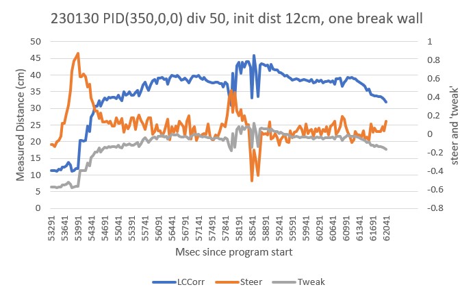
After this run I decided to push my luck and try a ‘two break’ wall configuration, again with a very small initial offset. Here’s the raw telemetry output, the corresponding Excel plot, and a short video showing the action.
|
1 2 3 4 5 6 7 8 9 10 11 12 13 14 15 16 17 18 19 20 21 22 23 24 25 26 27 28 29 30 31 32 33 34 35 36 37 38 39 40 41 42 43 44 45 46 47 48 49 50 51 52 53 54 55 56 57 58 59 60 61 62 63 64 65 66 67 68 69 70 71 72 73 74 75 76 77 78 79 80 81 82 83 84 85 86 87 88 89 90 91 92 93 94 95 96 97 98 99 100 101 102 103 104 105 106 107 108 109 110 111 112 113 114 115 116 117 118 119 120 121 122 123 124 125 126 127 128 129 130 131 132 133 134 135 136 137 138 139 140 141 142 143 144 145 146 147 148 149 150 151 152 153 154 155 156 157 158 159 160 161 162 163 164 165 166 167 168 169 170 171 172 173 174 175 176 177 178 179 180 181 182 183 184 185 186 187 188 189 190 |
Front Center Rear Steer 14.20 13.00 15.30 -0.11 14.20 13.80 15.20 -0.10 14.30 13.00 15.20 -0.08 WallE3_WallTrackTuning_V5.ino: TrackLeftWallOffset: Start tracking offset of 40.0 cm with Kp/Ki/Kd = 350.00 0.00 0.00 Msec LF LC LR Steer Deg Cos LCCorr Set Err SpinDeg WallE3_WallTrackTuning_V5.ino: In TrackLeftWallOffset: before while with errcode = NO_ANOMALIES Msec LF LC LR LCCorr Steer Tweak OffCm Err LastI LastD Out Lspd Rspd 26504 14.20 13.30 15.30 13.04 -0.11 -0.54 40.00 0.65 0.00 0.65 227.21 127 0 26554 14.10 12.80 15.20 12.55 -0.11 -0.55 40.00 0.66 0.00 0.01 230.64 127 0 26604 14.40 13.40 15.30 13.22 -0.09 -0.54 40.00 0.63 0.00 -0.03 218.93 127 0 26654 14.60 13.30 15.20 13.22 -0.06 -0.54 40.00 0.60 0.00 -0.03 208.44 127 0 26704 15.00 13.50 14.90 13.50 0.01 -0.53 40.00 0.52 0.00 -0.08 182.02 127 0 26754 15.20 13.70 14.90 13.68 0.03 -0.53 40.00 0.50 0.00 -0.02 173.74 127 0 26804 16.30 14.80 14.80 14.27 0.15 -0.51 40.00 0.36 0.00 -0.13 127.60 127 0 26854 18.20 15.60 15.00 13.28 0.32 -0.53 40.00 0.21 0.00 -0.15 75.02 127 0 26904 20.40 15.60 15.00 13.28 0.32 -0.53 40.00 0.21 0.00 0.00 75.02 127 0 26954 20.40 17.30 16.10 13.04 0.43 -0.54 40.00 0.11 0.00 -0.11 38.22 113 36 27004 23.00 19.90 18.00 13.67 0.50 -0.53 40.00 0.03 0.00 -0.08 9.28 84 65 27054 26.70 24.40 20.20 13.25 0.65 -0.53 40.00 -0.12 0.00 -0.14 -40.28 34 115 27104 29.90 28.40 23.10 14.63 0.68 -0.51 40.00 -0.17 0.00 -0.06 -60.42 14 127 27154 33.70 31.40 25.90 13.35 0.78 -0.53 40.00 -0.25 0.00 -0.07 -86.48 0 127 27204 35.20 35.30 29.00 20.18 0.62 -0.40 40.00 -0.22 0.00 0.02 -78.24 0 127 27254 37.00 36.00 30.30 18.88 0.67 -0.42 40.00 -0.25 0.00 -0.02 -86.67 0 127 27304 37.00 36.90 31.90 25.00 0.51 -0.30 40.00 -0.21 0.00 0.04 -73.49 1 127 27354 37.00 36.90 31.90 25.00 0.51 -0.30 40.00 -0.21 0.00 0.00 -73.49 1 127 27404 37.70 37.10 31.60 21.56 0.61 -0.37 40.00 -0.24 0.00 -0.03 -84.42 0 127 27454 36.60 37.30 32.20 27.77 0.44 -0.24 40.00 -0.20 0.00 0.05 -68.36 6 127 27504 35.30 35.60 31.40 28.15 0.39 -0.24 40.00 -0.15 0.00 0.04 -53.54 21 127 27554 35.20 35.30 32.10 30.35 0.31 -0.19 40.00 -0.12 0.00 0.04 -40.92 34 115 27604 34.50 34.00 31.60 29.77 0.29 -0.20 40.00 -0.09 0.00 0.03 -29.88 45 104 27654 33.80 34.10 32.00 32.37 0.18 -0.15 40.00 -0.03 0.00 0.06 -9.56 65 84 27704 34.00 33.80 32.50 32.59 0.15 -0.15 40.00 -0.00 0.00 0.03 -0.64 74 75 27754 34.30 34.60 32.50 33.36 0.15 -0.13 40.00 -0.02 0.00 -0.02 -6.04 68 81 27804 34.30 34.60 32.90 33.52 0.14 -0.13 40.00 -0.01 0.00 0.01 -3.63 71 78 27854 34.10 34.30 32.90 33.51 0.12 -0.13 40.00 0.01 0.00 0.02 3.45 78 71 27904 34.50 34.80 33.00 33.56 0.15 -0.13 40.00 -0.02 0.00 -0.03 -7.39 67 82 27954 34.50 34.50 33.70 34.14 0.08 -0.12 40.00 0.04 0.00 0.06 13.00 88 61 28004 34.60 34.80 33.60 34.24 0.10 -0.12 40.00 0.02 0.00 -0.02 5.33 80 69 28054 34.90 35.60 34.20 35.32 0.07 -0.09 40.00 0.02 0.00 0.01 8.28 83 66 28104 34.80 35.20 34.10 34.92 0.07 -0.10 40.00 0.03 0.00 0.01 11.06 86 63 28154 34.70 35.50 34.00 35.22 0.07 -0.10 40.00 0.03 0.00 -0.01 8.98 83 66 28204 34.70 35.50 34.00 35.22 0.07 -0.10 40.00 0.03 0.00 0.00 8.98 83 66 28254 34.70 35.20 33.80 34.74 0.09 -0.11 40.00 0.02 0.00 -0.01 5.33 80 69 28304 35.20 35.70 34.20 35.12 0.10 -0.10 40.00 -0.00 0.00 -0.02 -0.87 74 75 28354 35.30 37.00 34.40 36.52 0.09 -0.07 40.00 -0.02 0.00 -0.02 -7.11 67 82 28404 35.30 36.80 35.00 36.75 0.03 -0.07 40.00 0.04 0.00 0.06 12.28 87 62 28454 35.90 36.30 34.60 35.32 0.13 -0.09 40.00 -0.04 0.00 -0.07 -12.73 62 87 28504 36.10 36.50 35.00 35.79 0.11 -0.08 40.00 -0.03 0.00 0.01 -9.03 65 84 28554 36.10 36.40 35.20 35.92 0.09 -0.08 40.00 -0.01 0.00 0.02 -2.96 72 77 28604 36.10 36.70 35.40 36.41 0.07 -0.07 40.00 0.00 0.00 0.01 0.64 75 74 28654 35.40 36.80 34.90 36.65 0.05 -0.07 40.00 0.02 0.00 0.02 5.95 80 69 28704 35.20 37.10 35.20 37.10 0.00 -0.06 40.00 0.06 0.00 0.04 20.30 95 54 28754 35.50 37.20 35.40 37.19 0.01 -0.06 40.00 0.05 0.00 -0.01 16.14 91 58 28804 36.60 38.50 35.20 37.30 0.14 -0.05 40.00 -0.09 0.00 -0.13 -30.08 44 105 28854 36.80 39.30 36.10 38.99 0.07 -0.02 40.00 -0.05 0.00 0.04 -17.41 57 92 28904 40.20 41.80 35.80 31.12 0.44 -0.18 40.00 -0.26 0.00 -0.21 -91.81 0 127 28954 39.60 42.80 38.00 41.07 0.16 0.02 40.00 -0.18 0.00 0.08 -63.46 11 127 29004 42.20 45.00 38.90 37.94 0.33 -0.04 40.00 -0.29 0.00 -0.11 -101.10 0 127 29054 42.50 45.20 39.70 39.92 0.28 -0.00 40.00 -0.28 0.00 0.01 -97.46 0 127 29104 44.00 45.00 39.90 34.76 0.41 -0.10 40.00 -0.31 0.00 -0.03 -106.80 0 127 29154 43.40 46.90 40.30 40.32 0.31 0.01 40.00 -0.32 0.00 -0.01 -110.73 0 127 29204 43.60 45.60 40.60 39.57 0.30 -0.01 40.00 -0.29 0.00 0.03 -101.97 0 127 29254 44.40 45.10 41.70 40.17 0.27 0.00 40.00 -0.27 0.00 0.02 -95.72 0 127 29304 43.30 45.20 41.40 42.65 0.19 0.05 40.00 -0.24 0.00 0.03 -85.04 0 127 29354 44.10 45.50 41.00 39.11 0.31 -0.02 40.00 -0.29 0.00 -0.05 -102.30 0 127 29404 43.50 46.00 42.10 44.56 0.14 0.09 40.00 -0.23 0.00 0.06 -80.94 0 127 29454 42.60 45.70 42.00 45.23 0.08 0.10 40.00 -0.18 0.00 0.05 -64.58 10 127 29504 42.60 45.70 43.10 45.51 -0.05 0.11 40.00 -0.06 0.00 0.12 -21.10 53 96 29554 44.30 47.10 43.80 47.09 -0.01 0.14 40.00 -0.13 0.00 -0.07 -46.15 28 121 29604 45.70 49.90 49.20 41.22 -0.35 0.02 40.00 0.33 0.00 0.46 113.93 127 0 29654 46.60 51.10 51.30 36.58 -0.47 -0.07 40.00 0.54 0.00 0.21 188.42 127 0 29704 48.60 49.80 51.00 45.43 -0.24 0.11 40.00 0.13 0.00 -0.41 46.01 121 28 29754 44.40 48.10 49.00 34.89 -0.46 -0.10 40.00 0.56 0.00 0.43 196.74 127 0 29804 43.50 46.40 47.00 38.33 -0.35 -0.03 40.00 0.38 0.00 -0.18 134.17 127 0 29854 42.40 44.60 43.40 43.88 -0.10 0.08 40.00 0.02 0.00 -0.36 7.84 82 67 29904 41.30 43.50 42.80 41.94 -0.15 0.04 40.00 0.11 0.00 0.09 38.89 113 36 29954 40.40 43.20 40.50 43.19 -0.01 0.06 40.00 -0.05 0.00 -0.16 -18.85 56 93 30004 39.00 41.50 39.10 41.49 -0.01 0.03 40.00 -0.02 0.00 0.03 -6.95 68 81 30054 39.00 40.20 39.80 39.78 -0.08 -0.00 40.00 0.08 0.00 0.10 29.52 104 45 30104 37.80 39.90 38.20 39.80 -0.04 -0.00 40.00 0.04 0.00 -0.04 15.43 90 59 30154 37.60 40.00 38.50 39.48 -0.09 -0.01 40.00 0.10 0.00 0.06 35.17 110 39 30204 36.60 38.80 37.90 37.75 -0.13 -0.04 40.00 0.17 0.00 0.07 61.24 127 13 30254 36.50 38.30 36.90 38.20 -0.04 -0.04 40.00 0.08 0.00 -0.10 26.60 101 48 30304 35.30 38.60 37.00 36.84 -0.17 -0.06 40.00 0.23 0.00 0.16 81.61 127 0 30354 36.00 37.00 36.80 36.62 -0.08 -0.07 40.00 0.15 0.00 -0.09 51.69 126 23 30404 35.40 36.80 35.90 36.65 -0.05 -0.07 40.00 0.12 0.00 -0.03 40.95 115 34 30454 34.00 36.10 35.20 35.27 -0.12 -0.09 40.00 0.21 0.00 0.10 75.14 127 0 30504 34.80 35.50 34.60 35.48 0.02 -0.09 40.00 0.07 0.00 -0.14 24.66 99 50 30554 34.30 35.80 34.00 35.75 0.03 -0.09 40.00 0.06 0.00 -0.02 19.27 94 55 30604 34.90 36.30 34.20 35.92 0.08 -0.08 40.00 0.00 0.00 -0.05 0.53 75 74 30654 34.30 36.40 34.70 36.31 -0.04 -0.07 40.00 0.11 0.00 0.11 39.86 114 35 30704 35.60 36.50 34.50 35.79 0.11 -0.08 40.00 -0.03 0.00 -0.14 -9.03 65 84 30754 35.40 37.40 35.10 37.35 0.03 -0.05 40.00 0.02 0.00 0.05 8.08 83 66 30804 36.50 37.90 35.40 37.16 0.11 -0.06 40.00 -0.05 0.00 -0.08 -18.64 56 93 30854 35.80 38.50 35.80 38.50 0.00 -0.03 40.00 0.03 0.00 0.08 10.50 85 64 30904 36.40 38.40 35.20 37.51 0.12 -0.05 40.00 -0.07 0.00 -0.10 -24.59 50 99 30954 36.00 39.00 35.80 38.10 0.12 -0.04 40.00 -0.08 0.00 -0.01 -28.69 46 103 31004 38.20 39.10 36.60 37.52 0.16 -0.05 40.00 -0.11 0.00 -0.03 -38.61 36 113 31054 37.50 39.20 36.50 38.57 0.10 -0.03 40.00 -0.07 0.00 0.04 -24.97 50 99 31104 37.80 40.00 36.80 39.35 0.10 -0.01 40.00 -0.09 0.00 -0.02 -30.48 44 105 31154 38.60 40.30 37.90 39.98 0.07 -0.00 40.00 -0.07 0.00 0.02 -24.36 50 99 31204 37.10 39.90 37.70 39.67 -0.06 -0.01 40.00 0.07 0.00 0.14 23.33 98 51 31254 38.40 40.40 37.40 39.75 0.10 -0.01 40.00 -0.09 0.00 -0.16 -33.24 41 108 31304 38.00 40.10 37.10 39.57 0.09 -0.01 40.00 -0.08 0.00 0.01 -28.52 46 103 31354 38.60 39.90 37.20 38.65 0.14 -0.03 40.00 -0.11 0.00 -0.03 -39.57 35 114 31404 38.80 40.30 37.70 39.52 0.11 -0.01 40.00 -0.10 0.00 0.01 -35.11 39 110 31454 39.00 41.10 38.30 40.77 0.07 0.02 40.00 -0.09 0.00 0.01 -29.91 45 104 31504 39.00 40.70 38.10 40.17 0.09 0.00 40.00 -0.09 0.00 -0.01 -32.67 42 107 31554 39.40 41.00 37.20 37.94 0.22 -0.04 40.00 -0.18 0.00 -0.09 -62.60 12 127 31604 38.10 40.50 38.50 40.39 -0.04 0.01 40.00 0.03 0.00 0.21 11.24 86 63 31654 37.80 40.50 38.10 40.44 -0.03 0.01 40.00 0.02 0.00 -0.01 7.42 82 67 31704 38.40 40.70 39.00 40.46 -0.06 0.01 40.00 0.05 0.00 0.03 17.77 92 57 31754 39.00 40.30 38.50 40.14 0.05 0.00 40.00 -0.05 0.00 -0.10 -18.45 56 93 31804 39.20 40.10 38.00 39.17 0.12 -0.02 40.00 -0.10 0.00 -0.05 -36.21 38 111 31854 38.80 41.20 37.70 40.40 0.11 0.01 40.00 -0.12 0.00 -0.01 -41.29 33 116 31904 38.30 40.20 38.20 40.19 0.01 0.00 40.00 -0.01 0.00 0.10 -4.85 70 79 31954 37.30 39.90 37.90 39.67 -0.06 -0.01 40.00 0.07 0.00 0.08 23.33 98 51 32004 35.90 37.30 38.10 34.52 -0.22 -0.11 40.00 0.33 0.00 0.26 115.37 127 0 32054 34.70 36.90 36.80 34.38 -0.21 -0.11 40.00 0.32 0.00 -0.01 112.84 127 0 32104 33.30 35.10 35.80 31.77 -0.25 -0.16 40.00 0.41 0.00 0.09 145.08 127 0 32154 31.90 33.60 34.40 30.42 -0.25 -0.19 40.00 0.44 0.00 0.03 154.59 127 0 32204 30.60 30.90 32.30 29.49 -0.17 -0.21 40.00 0.38 0.00 -0.06 133.06 127 0 32254 29.20 30.30 29.60 30.22 -0.04 -0.20 40.00 0.24 0.00 -0.14 82.45 127 0 32304 28.50 27.50 28.50 27.50 0.00 -0.25 40.00 0.25 0.00 0.01 87.50 127 0 32354 27.30 26.90 28.10 26.62 -0.08 -0.27 40.00 0.35 0.00 0.10 121.65 127 0 32404 25.90 26.00 26.40 25.89 -0.05 -0.28 40.00 0.33 0.00 -0.02 116.24 127 0 32454 25.10 25.10 25.00 25.10 0.01 -0.30 40.00 0.29 0.00 -0.04 100.83 127 0 32504 25.30 25.10 24.60 24.90 0.07 -0.30 40.00 0.23 0.00 -0.06 81.20 127 0 32554 25.40 25.10 24.60 24.90 0.07 -0.30 40.00 0.23 0.00 0.00 81.20 127 0 32604 25.40 25.60 24.20 25.01 0.12 -0.30 40.00 0.18 0.00 -0.05 62.94 127 12 32654 26.30 26.10 24.60 24.91 0.17 -0.30 40.00 0.13 0.00 -0.05 46.12 121 28 32704 27.90 27.80 25.30 24.97 0.26 -0.30 40.00 0.04 0.00 -0.09 14.23 89 60 32754 30.40 30.70 26.80 25.09 0.36 -0.30 40.00 -0.06 0.00 -0.10 -21.66 53 96 32804 33.20 33.50 28.80 24.94 0.44 -0.30 40.00 -0.14 0.00 -0.08 -48.56 26 123 32854 35.70 36.40 30.70 25.01 0.50 -0.30 40.00 -0.20 0.00 -0.06 -70.08 4 127 32904 37.10 39.10 33.60 32.30 0.35 -0.15 40.00 -0.20 0.00 0.00 -68.61 6 127 32954 39.10 40.20 34.30 28.39 0.48 -0.23 40.00 -0.25 0.00 -0.05 -86.76 0 127 33004 39.10 40.20 34.30 28.39 0.48 -0.23 40.00 -0.25 0.00 0.00 -86.76 0 127 33054 39.20 41.50 36.00 35.34 0.32 -0.09 40.00 -0.23 0.00 0.02 -79.36 0 127 33104 39.60 42.00 35.30 31.66 0.43 -0.17 40.00 -0.26 0.00 -0.04 -92.11 0 127 33154 38.80 40.30 36.00 35.60 0.28 -0.09 40.00 -0.19 0.00 0.07 -67.17 7 127 33204 39.50 40.10 36.10 33.47 0.34 -0.13 40.00 -0.21 0.00 -0.02 -73.30 1 127 33254 39.40 41.50 35.80 33.92 0.36 -0.12 40.00 -0.24 0.00 -0.03 -83.46 0 127 33304 38.00 40.00 37.40 39.77 0.06 -0.00 40.00 -0.06 0.00 0.18 -19.36 55 94 33354 38.20 39.50 35.80 36.03 0.24 -0.08 40.00 -0.16 0.00 -0.11 -56.22 18 127 33404 37.80 39.90 35.80 36.40 0.24 -0.07 40.00 -0.17 0.00 -0.01 -58.77 16 127 33454 37.70 40.00 37.10 39.77 0.06 -0.00 40.00 -0.06 0.00 0.11 -19.36 55 94 33504 37.90 40.40 37.10 40.16 0.06 0.00 40.00 -0.06 0.00 -0.01 -22.14 52 97 33554 37.50 39.60 38.40 39.08 -0.09 -0.02 40.00 0.11 0.00 0.17 37.93 112 37 33604 37.80 40.30 38.40 39.77 -0.09 -0.00 40.00 0.09 0.00 -0.01 33.09 108 41 33654 37.80 40.30 38.90 39.52 -0.11 -0.01 40.00 0.12 0.00 0.03 41.89 116 33 33704 37.70 39.80 38.30 39.57 -0.06 -0.01 40.00 0.07 0.00 -0.05 24.03 99 50 33754 36.20 39.50 38.70 35.76 -0.25 -0.08 40.00 0.33 0.00 0.27 117.20 127 0 33804 35.90 39.10 36.90 38.47 -0.10 -0.03 40.00 0.13 0.00 -0.20 45.71 120 29 33854 35.70 36.90 36.30 36.68 -0.06 -0.07 40.00 0.13 0.00 -0.00 44.21 119 30 33904 34.60 36.70 35.80 35.85 -0.12 -0.08 40.00 0.20 0.00 0.08 71.04 127 3 33954 35.00 36.10 33.70 35.12 0.13 -0.10 40.00 -0.03 0.00 -0.24 -11.37 63 86 34004 34.90 36.60 33.40 35.29 0.15 -0.09 40.00 -0.06 0.00 -0.02 -19.54 55 94 34054 34.90 36.60 33.40 35.29 0.15 -0.09 40.00 -0.06 0.00 0.00 -19.54 55 94 34104 35.10 37.50 34.60 37.35 0.05 -0.05 40.00 0.00 0.00 0.06 1.07 76 73 34154 35.10 37.50 34.60 37.35 0.05 -0.05 40.00 0.00 0.00 0.00 1.07 76 73 34204 35.90 37.70 34.50 36.52 0.14 -0.07 40.00 -0.07 0.00 -0.07 -24.65 50 99 34254 36.50 37.90 34.80 36.17 0.17 -0.08 40.00 -0.09 0.00 -0.02 -32.71 42 107 34304 36.50 38.90 34.70 36.92 0.18 -0.06 40.00 -0.12 0.00 -0.02 -41.45 33 116 34354 38.10 40.30 35.50 36.19 0.26 -0.08 40.00 -0.18 0.00 -0.07 -64.36 10 127 34404 37.70 39.90 36.70 39.26 0.10 -0.01 40.00 -0.09 0.00 0.10 -29.79 45 104 34454 38.30 41.10 36.80 39.63 0.15 -0.01 40.00 -0.14 0.00 -0.06 -49.92 25 124 34504 38.10 40.70 37.10 40.04 0.10 0.00 40.00 -0.10 0.00 0.04 -35.30 39 110 34554 39.00 41.20 36.70 37.86 0.23 -0.04 40.00 -0.19 0.00 -0.09 -65.51 9 127 34604 39.00 41.20 36.70 37.86 0.23 -0.04 40.00 -0.19 0.00 0.00 -65.51 9 127 34654 39.00 41.50 38.40 41.26 0.06 0.03 40.00 -0.09 0.00 0.10 -29.80 45 104 34704 39.60 41.10 38.50 40.30 0.11 0.01 40.00 -0.12 0.00 -0.03 -40.60 34 115 34754 38.80 40.90 39.30 40.73 -0.05 0.01 40.00 0.04 0.00 0.15 12.37 87 62 34804 39.10 41.00 38.30 40.57 0.08 0.01 40.00 -0.09 0.00 -0.13 -32.02 42 107 34854 39.20 40.80 39.00 40.77 0.02 0.02 40.00 -0.04 0.00 0.06 -12.41 62 87 34904 37.70 41.70 39.70 39.10 -0.20 -0.02 40.00 0.22 0.00 0.25 76.27 127 0 34954 38.70 40.50 38.80 40.49 -0.01 0.01 40.00 0.00 0.00 -0.22 0.05 75 74 35004 37.60 39.50 38.00 39.40 -0.04 -0.01 40.00 0.05 0.00 0.05 18.22 93 56 35054 36.60 38.70 38.80 35.81 -0.22 -0.08 40.00 0.30 0.00 0.25 106.30 127 0 35104 35.90 38.00 37.10 37.12 -0.12 -0.06 40.00 0.18 0.00 -0.13 62.15 127 12 35154 35.80 37.20 35.20 36.98 0.06 -0.06 40.00 0.00 0.00 -0.18 0.12 75 74 35204 33.80 36.30 34.80 35.71 -0.10 -0.09 40.00 0.19 0.00 0.19 65.00 127 10 35254 33.80 36.00 33.50 35.95 0.03 -0.08 40.00 0.05 0.00 -0.13 17.87 92 57 35304 33.10 34.50 33.50 34.45 0.03 -0.11 40.00 0.08 0.00 0.03 28.35 103 46 |
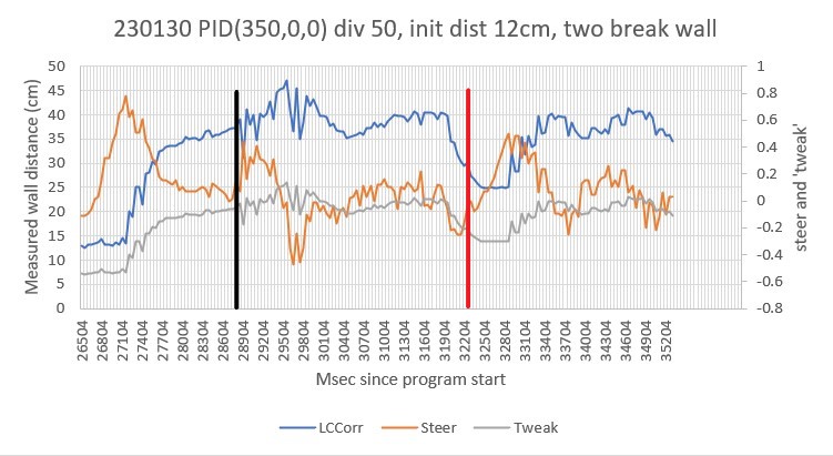
From the above it is pretty clear that PID(350,0,0) and ‘tweak’ divisor 50 does a very good job of tracking a straight, one-break or two-break wall at a defined offset distance. In addition it is pretty clear that this configuration does not require a separate ‘offset capture’ function – it does just fine all by itself. I guess I’m a little bummed out that I spent so much time ‘perfecting’ (to the degree that anything I do can be said to be ‘perfect’) the capture function.
23 July 2023 Update:
I have been trying to address the tendency of WallE3 to oscillate back and forth after navigating past the 45º break from the entrance hallway into the kitchen, and I kept getting the feeling I had already solved this problem at least once before. I searched through my older posts and found this one, which clearly shows much better performance than I was now seeing. After carefully perusing the above data, I finally figured out the difference; the above runs used a 50mSec interval, and I was currently using a 100mSec interval – oops!
I changed my current code to 50mSec, and ‘sure nuff’ WallE3’s wall tracking performance around breaks improved dramatically – yay!
This episode proves once again the value of copious documentation – you never know when you will need advice from your former self!
After changing the PID update interval to 50 vs 100 mSec, I made a few runs on my ’45º break’ wall configuration with PID = (350,0,0), (350,0,10), (350,0,20), and (350,0,30). As shown in the following three short videos, both the (350,0,10) and (350,0,20) produced better tracking performance, but the (350,0,30) was definitely inferior.
After these tests, I edited WallE3_Complete_V3 to use PID = (350,0,20) with a 50mSec interval.