// Implementation of Sebastian Madgwick's "...efficient orientation filter for... inertial/magnetic sensor arrays"
// (see http://www.x-io.co.uk/category/open-source/ for examples and more details)
// which fuses acceleration and rotation rate to produce a quaternion-based estimate of relative
// device orientation -- which can be converted to yaw, pitch, and roll. Useful for stabilizing quadcopters, etc.
// The performance of the orientation filter is at least as good as conventional Kalman-based filtering algorithms
// but is much less computationally intensive---it can be performed on a 3.3 V Pro Mini operating at 8 MHz!
void Class_MPU9250BasicAHRS::MadgwickQuaternionUpdate(float ax, float ay, float az, float gx, float gy, float gz)
//void Class_MPU9250BasicAHRS::MadgwickQuaternionUpdate(float ax, float ay, float az, float gx, float gy, float gz, float q_array[4], float delta_t)
{
float q1 = q[0], q2 = q[1], q3 = q[2], q4 = q[3]; // short name local variable for readability
//float q1 = q_array[0], q2 = q_array[1], q3 = q_array[2], q4 = q_array[3]; // short name local variable for readability
float norm; // vector norm
float f1, f2, f3; // objetive funcyion elements
float J_11or24, J_12or23, J_13or22, J_14or21, J_32, J_33; // objective function Jacobian elements
float qDot1, qDot2, qDot3, qDot4;
float hatDot1, hatDot2, hatDot3, hatDot4;
float gerrx, gerry, gerrz, gbiasx, gbiasy, gbiasz; // gyro bias error
// Auxiliary variables to avoid repeated arithmetic
float _halfq1 = 0.5f * q1;
float _halfq2 = 0.5f * q2;
float _halfq3 = 0.5f * q3;
float _halfq4 = 0.5f * q4;
float _2q1 = 2.0f * q1;
float _2q2 = 2.0f * q2;
float _2q3 = 2.0f * q3;
float _2q4 = 2.0f * q4;
//04/24/18 bugfix: these vars aren't used in 6DOF version
//float _2q1q3 = 2.0f * q1 * q3;
//float _2q3q4 = 2.0f * q3 * q4;
// Normalise accelerometer measurement
norm = sqrt(ax * ax + ay * ay + az * az);
if (norm == 0.0f) return; // handle NaN
norm = 1.0f / norm;
ax *= norm;
ay *= norm;
az *= norm;
// Compute the objective function and Jacobian
f1 = _2q2 * q4 - _2q1 * q3 - ax;
f2 = _2q1 * q2 + _2q3 * q4 - ay;
f3 = 1.0f - _2q2 * q2 - _2q3 * q3 - az;
J_11or24 = _2q3;
J_12or23 = _2q4;
J_13or22 = _2q1;
J_14or21 = _2q2;
J_32 = 2.0f * J_14or21;
J_33 = 2.0f * J_11or24;
// Compute the gradient (matrix multiplication)
hatDot1 = J_14or21 * f2 - J_11or24 * f1;
hatDot2 = J_12or23 * f1 + J_13or22 * f2 - J_32 * f3;
hatDot3 = J_12or23 * f2 - J_33 * f3 - J_13or22 * f1;
hatDot4 = J_14or21 * f1 + J_11or24 * f2;
// Normalize the gradient
norm = sqrt(hatDot1 * hatDot1 + hatDot2 * hatDot2 + hatDot3 * hatDot3 + hatDot4 * hatDot4);
hatDot1 /= norm;
hatDot2 /= norm;
hatDot3 /= norm;
hatDot4 /= norm;
// Compute estimated gyroscope biases
gerrx = _2q1 * hatDot2 - _2q2 * hatDot1 - _2q3 * hatDot4 + _2q4 * hatDot3;
gerry = _2q1 * hatDot3 + _2q2 * hatDot4 - _2q3 * hatDot1 - _2q4 * hatDot2;
gerrz = _2q1 * hatDot4 - _2q2 * hatDot3 + _2q3 * hatDot2 - _2q4 * hatDot1;
// Compute and remove gyroscope biases
//04/24/18 bugfix: gbias vars are unitialized here
//gbiasx += gerrx * deltat_sec * zeta;
//gbiasy += gerry * deltat_sec * zeta;
//gbiasz += gerrz * deltat_sec * zeta;
gbiasx = gerrx * deltat_sec * zeta;
gbiasy = gerry * deltat_sec * zeta;
gbiasz = gerrz * deltat_sec * zeta;
gx -= gbiasx;
gy -= gbiasy;
gz -= gbiasz;
// Compute the quaternion derivative
qDot1 = -_halfq2 * gx - _halfq3 * gy - _halfq4 * gz;
qDot2 = _halfq1 * gx + _halfq3 * gz - _halfq4 * gy;
qDot3 = _halfq1 * gy - _halfq2 * gz + _halfq4 * gx;
qDot4 = _halfq1 * gz + _halfq2 * gy - _halfq3 * gx;
// Compute then integrate estimated quaternion derivative
q1 += (qDot1 - (beta * hatDot1)) * deltat_sec;
q2 += (qDot2 - (beta * hatDot2)) * deltat_sec;
q3 += (qDot3 - (beta * hatDot3)) * deltat_sec;
q4 += (qDot4 - (beta * hatDot4)) * deltat_sec;
// Normalize the quaternion
norm = sqrt(q1 * q1 + q2 * q2 + q3 * q3 + q4 * q4); // normalise quaternion
norm = 1.0f / norm;
q[0] = q1 * norm;
q[1] = q2 * norm;
q[2] = q3 * norm;
q[3] = q4 * norm;
}
float Class_MPU9250BasicAHRS::GetIMUHeadingDeg()
{
// If intPin goes high, all data registers have new data
//if (readByte(MPU9250_ADDRESS, INT_STATUS) & 0x01)
{ // On interrupt, check if data ready interrupt
readAccelData(accelCount); // Read the x/y/z adc values
getAres();
// Now we'll calculate the accleration value into actual g's
ax = (float)accelCount[0] * aRes; // - accelBias[0]; // get actual g value, this depends on scale being set
ay = (float)accelCount[1] * aRes; // - accelBias[1];
az = (float)accelCount[2] * aRes; // - accelBias[2];
readGyroData(gyroCount); // Read the x/y/z adc values
getGres();
// Calculate the gyro value into actual degrees per second
gx = (float)gyroCount[0] * gRes; // get actual gyro value, this depends on scale being set
gy = (float)gyroCount[1] * gRes;
gz = (float)gyroCount[2] * gRes;
#ifndef NO_MAG
readMagData(magCount); // Read the x/y/z adc values
getMres();
magbias[0] = +470.; // User environmental x-axis correction in milliGauss, should be automatically calculated
magbias[1] = +120.; // User environmental x-axis correction in milliGauss
magbias[2] = +125.; // User environmental x-axis correction in milliGauss
// Calculate the magnetometer values in milliGauss
// Include factory calibration per data sheet and user environmental corrections
mx = (float)magCount[0] * mRes*magCalibration[0] - magbias[0]; // get actual magnetometer value, this depends on scale being set
my = (float)magCount[1] * mRes*magCalibration[1] - magbias[1];
mz = (float)magCount[2] * mRes*magCalibration[2] - magbias[2];
#endif // !NO_MAG
}
Now = micros();
deltat_sec = ((Now - lastUpdate) / 1000000.0f); // set integration time by time elapsed since last filter update
lastUpdate = Now;
sum += deltat_sec; // sum for averaging filter update rate
sumCount++;
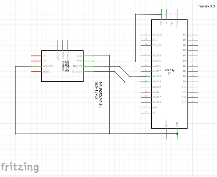
// Sensors x (y)-axis of the accelerometer is aligned with the y (x)-axis of the magnetometer;
// the magnetometer z-axis (+ down) is opposite to z-axis (+ up) of accelerometer and gyro!
// We have to make some allowance for this orientationmismatch in feeding the output to the quaternion filter.
// For the MPU-9250, we have chosen a magnetic rotation that keeps the sensor forward along the x-axis just like
// in the LSM9DS0 sensor. This rotation can be modified to allow any convenient orientation convention.
// This is ok by aircraft orientation standards!
// Pass gyro rate as rad/s
#ifndef NO_MAG
MadgwickQuaternionUpdate(ax, ay, az, gx*PI / 180.0f, gy*PI / 180.0f, gz*PI / 180.0f, my, mx, mz);
// MahonyQuaternionUpdate(ax, ay, az, gx*PI/180.0f, gy*PI/180.0f, gz*PI/180.0f, my, mx, mz);
#else
//Serial.printf("q = {%4.2f, %4.2f, %4.2f, %4.2f, deltat_ms = %2.4f\n", q[0], q[1], q[2], q[3], deltat_sec*1000);
//experiment with multiple iterations on quat update
//for (size_t i = 0; i < 10; i++)
{
MadgwickQuaternionUpdate(ax, ay, az, gx*PI / 180.0f, gy*PI / 180.0f, gz*PI / 180.0f);
}
//MadgwickQuaternionUpdate(ax, ay, az, gx*PI / 180.0f, gy*PI / 180.0f, gz*PI / 180.0f, q, deltat_sec);
#endif // !NO_MAG
if (!AHRS)
{
delt_t = millis() - count;
if (delt_t > 500)
{
if (SerialDebug) {
// Print acceleration values in milligs!
Serial.print("X-acceleration: "); Serial.print(1000 * ax); Serial.print(" mg ");
Serial.print("Y-acceleration: "); Serial.print(1000 * ay); Serial.print(" mg ");
Serial.print("Z-acceleration: "); Serial.print(1000 * az); Serial.println(" mg ");
// Print gyro values in degree/sec
Serial.print("X-gyro rate: "); Serial.print(gx, 3); Serial.print(" degrees/sec ");
Serial.print("Y-gyro rate: "); Serial.print(gy, 3); Serial.print(" degrees/sec ");
Serial.print("Z-gyro rate: "); Serial.print(gz, 3); Serial.println(" degrees/sec");
#ifndef NO_MAG
// Print mag values in degree/sec
Serial.print("X-mag field: "); Serial.print(mx); Serial.print(" mG ");
Serial.print("Y-mag field: "); Serial.print(my); Serial.print(" mG ");
Serial.print("Z-mag field: "); Serial.print(mz); Serial.println(" mG");
tempCount = readTempData(); // Read the adc values
temperature = ((float)tempCount) / 333.87 + 21.0; // Temperature in degrees Centigrade
// Print temperature in degrees Centigrade
Serial.print("Temperature is "); Serial.print(temperature, 1); Serial.println(" degrees C"); // Print T values to tenths of s degree C
#endif // !NO_MAG
}
count = millis();
}
}
else
{
// Serial print and/or display at 0.5 s rate independent of data rates
delt_t = millis() - count;
//if (delt_t > 500)
{ // update LCD once per half-second independent of read rate
if (SerialDebug) {
Serial.print("ax = "); Serial.print((int)1000 * ax);
Serial.print(" ay = "); Serial.print((int)1000 * ay);
Serial.print(" az = "); Serial.print((int)1000 * az); Serial.println(" mg");
Serial.print("gx = "); Serial.print(gx, 2);
Serial.print(" gy = "); Serial.print(gy, 2);
Serial.print(" gz = "); Serial.print(gz, 2); Serial.println(" deg/s");
#ifndef NO_MAG
Serial.print("mx = "); Serial.print((int)mx);
Serial.print(" my = "); Serial.print((int)my);
Serial.print(" mz = "); Serial.print((int)mz); Serial.println(" mG");
#endif // !NO_MAG
Serial.print("q0 = "); Serial.print(q[0]);
Serial.print(" qx = "); Serial.print(q[1]);
Serial.print(" qy = "); Serial.print(q[2]);
Serial.print(" qz = "); Serial.println(q[3]);
}
// Define output variables from updated quaternion---these are Tait-Bryan angles, commonly used in aircraft orientation.
// In this coordinate system, the positive z-axis is down toward Earth.
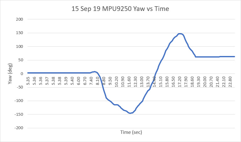
// Yaw is the angle between Sensor x-axis and Earth magnetic North (or true North if corrected for local declination, looking down on the sensor positive yaw is counterclockwise.
// Pitch is angle between sensor x-axis and Earth ground plane, toward the Earth is positive, up toward the sky is negative.
// Roll is angle between sensor y-axis and Earth ground plane, y-axis up is positive roll.
// These arise from the definition of the homogeneous rotation matrix constructed from quaternions.
// Tait-Bryan angles as well as Euler angles are non-commutative; that is, the get the correct orientation the rotations must be
// applied in the correct order which for this configuration is yaw, pitch, and then roll.
// For more see http://en.wikipedia.org/wiki/Conversion_between_quaternions_and_Euler_angles which has additional links.
yaw = atan2(2.0f * (q[1] * q[2] + q[0] * q[3]), q[0] * q[0] + q[1] * q[1] - q[2] * q[2] - q[3] * q[3]);
pitch = -asin(2.0f * (q[1] * q[3] - q[0] * q[2]));
roll = atan2(2.0f * (q[0] * q[1] + q[2] * q[3]), q[0] * q[0] - q[1] * q[1] - q[2] * q[2] + q[3] * q[3]);
pitch *= 180.0f / PI;
yaw *= 180.0f / PI;
//yaw -= 13.8; // Declination at Danville, California is 13 degrees 48 minutes and 47 seconds on 2014-04-04
roll *= 180.0f / PI;
if (SerialDebug) {
Serial.print("Yaw, Pitch, Roll: ");
Serial.print(yaw, 2);
Serial.print(", ");
Serial.print(pitch, 2);
Serial.print(", ");
Serial.println(roll, 2);
Serial.print("rate = "); Serial.print((float)sumCount / sum, 2); Serial.println(" Hz");
}
//Serial.printf("%3.2f\t%3.2f\t%3.2f\n", yaw, pitch, roll);
// With these settings the filter is updating at a ~145 Hz rate using the Madgwick scheme and
// >200 Hz using the Mahony scheme even though the display refreshes at only 2 Hz.
// The filter update rate is determined mostly by the mathematical steps in the respective algorithms,
// the processor speed (8 MHz for the 3.3V Pro Mini), and the magnetometer ODR:
// an ODR of 10 Hz for the magnetometer produce the above rates, maximum magnetometer ODR of 100 Hz produces
// filter update rates of 36 - 145 and ~38 Hz for the Madgwick and Mahony schemes, respectively.
// This is presumably because the magnetometer read takes longer than the gyro or accelerometer reads.
// This filter update rate should be fast enough to maintain accurate platform orientation for
// stabilization control of a fast-moving robot or quadcopter. Compare to the update rate of 200 Hz
// produced by the on-board Digital Motion Processor of Invensense's MPU6050 6 DoF and MPU9150 9DoF sensors.
// The 3.3 V 8 MHz Pro Mini is doing pretty well!
digitalWrite(myLed, !digitalRead(myLed));
count = millis();
sumCount = 0;
sum = 0;
}
}
return yaw;
}